

Unlocking the Power of Drop Down Lists in Excel
Microsoft Excel, a ubiquitous tool in offices and homes alike, offers a vast array of features designed to streamline data management and analysis. Among these, the drop down list stands out as a particularly useful function. It simplifies data entry, reduces errors, and enhances the overall usability of your spreadsheets. But beyond the basics, drop down lists can be further customized with color-coding, adding another layer of visual organization and clarity. This comprehensive guide will walk you through the process of creating and enhancing drop down lists in Excel, ensuring you can leverage this feature to its fullest potential.
Why Use Drop Down Lists?
Before diving into the how-to, let’s understand why drop down lists are so valuable. Imagine you’re managing a sales database. Instead of manually typing in the region for each sale (e.g., North, South, East, West), you can create a drop down list containing these options. This eliminates the risk of typos (e.g., Nortth) and ensures consistency in your data. Furthermore, drop down lists provide a controlled vocabulary, making data analysis and reporting much more reliable. Think about the time saved and the frustration avoided! It’s a win-win.
- Data Integrity: Ensures consistent and accurate data entry.
- Efficiency: Speeds up data entry process.
- User-Friendliness: Simplifies data input for users of all skill levels.
- Data Analysis: Facilitates easier sorting, filtering, and analysis.
In essence, drop down lists transform your spreadsheets from simple data repositories into powerful, user-friendly tools.
Creating a Basic Drop Down List in Excel
Let’s start with the fundamentals. Creating a basic drop down list in Excel is surprisingly straightforward. Here’s a step-by-step guide:
Step 1: Prepare Your Data Source
The foundation of any drop down list is the data it draws from. This data can be a simple list of items, a range of cells, or even a named range. For our example, let’s create a list of departments in a company: Marketing, Sales, Engineering, HR, and Finance. You can type these into a separate sheet or a dedicated area within your current sheet. Just ensure that the list is contiguous (no blank cells in between).
Step 2: Select the Target Cell(s)
Now, identify the cell(s) where you want the drop down list to appear. This is where users will select their options. Click on the cell to select it. If you want the same drop down list to apply to multiple cells, you can select a range of cells by clicking and dragging.
Step 3: Access Data Validation
This is where the magic happens. Go to the ‘Data’ tab on the Excel ribbon. In the ‘Data Tools’ group, click on ‘Data Validation’. This will open the Data Validation dialog box.
Step 4: Configure Data Validation Settings
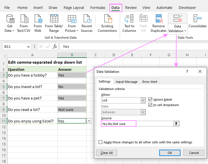
In the Data Validation dialog box, you’ll see three tabs: ‘Settings’, ‘Input Message’, and ‘Error Alert’. We’ll focus on the ‘Settings’ tab for now. In the ‘Allow’ dropdown, select ‘List’. This tells Excel that we want to create a drop down list.
Next, in the ‘Source’ field, specify the range of cells containing your data source (the list of departments we created earlier). You can either type the cell range directly (e.g., Sheet2!A1:A5) or click the small spreadsheet icon next to the ‘Source’ field to select the range using your mouse. Selecting with the mouse is often easier and less prone to errors.
Ensure that the ‘In-cell dropdown’ checkbox is checked. This is what actually creates the drop down arrow in the cell. Finally, click ‘OK’ to apply the data validation rule.
Step 5: Test Your Drop Down List
That’s it! You should now see a small arrow appear next to the cell(s) you selected. Click on the arrow to reveal the drop down list containing your departments. Select an option to populate the cell with the chosen value. Congratulations, you’ve created your first drop down list in Excel!
Advanced Drop Down List Techniques
Now that you’ve mastered the basics, let’s explore some advanced techniques to enhance your drop down lists and make them even more powerful.
Using Named Ranges
Instead of directly referencing cell ranges in the ‘Source’ field, you can use named ranges. A named range is simply a descriptive name assigned to a range of cells. This makes your formulas and data validation rules more readable and easier to maintain. If the underlying data changes (e.g., you add a new department), you only need to update the named range, and the drop down list will automatically reflect the changes.
To create a named range, select the range of cells containing your data source. Then, in the ‘Name Box’ (located to the left of the formula bar), type a descriptive name for the range (e.g., ‘Departments’) and press Enter. Now, in the Data Validation dialog box, you can simply enter =Departments in the ‘Source’ field. This is much cleaner and more understandable than a direct cell reference.
Creating Dependent Drop Down Lists
A dependent drop down list (also known as a cascading drop down list) is a drop down list whose options depend on the value selected in another drop down list. This is useful for creating hierarchical data entry systems. For example, you might have a first drop down list for ‘Country’ and a second drop down list for ‘City’, where the cities displayed in the second list depend on the country selected in the first list.
Creating dependent drop down lists requires a bit more setup, involving named ranges and the INDIRECT function. The basic idea is to create a table where each row represents a category from the first drop down list, and each column contains the corresponding options for the second drop down list. Then, you use the INDIRECT function to dynamically reference the correct column based on the value selected in the first drop down list.
While the specific steps can be a bit complex, numerous online tutorials and resources can guide you through the process. Search for “Excel dependent drop down list” to find detailed instructions and examples.
Using Drop Down Lists with Formulas
Drop down lists can be seamlessly integrated with Excel formulas to create dynamic calculations and reports. For example, you could use a drop down list to select a product category and then use a SUMIF formula to calculate the total sales for that category. The formula would automatically update whenever you select a different category from the drop down list.
This allows you to create interactive dashboards and reports that respond to user input, providing a powerful way to explore and analyze your data.
Adding Color to Drop Down Lists: A Visual Enhancement
Now, let’s move on to the exciting part: adding color to your drop down lists. While Excel doesn’t directly support color-coding within the drop down list itself, we can achieve a similar effect using conditional formatting. This involves applying formatting rules to the cells containing the drop down list based on the selected value.
Step 1: Select the Target Cells
As before, select the cell(s) containing the drop down list that you want to color-code.
Step 2: Access Conditional Formatting
Go to the ‘Home’ tab on the Excel ribbon. In the ‘Styles’ group, click on ‘Conditional Formatting’. This will open a menu of options.
Step 3: Create a New Rule
Select ‘New Rule…’ from the Conditional Formatting menu. This will open the New Formatting Rule dialog box.
Step 4: Choose a Rule Type
In the New Formatting Rule dialog box, select ‘Use a formula to determine which cells to format’. This allows us to define a custom formula that determines when the formatting should be applied.
Step 5: Enter the Formula
This is the crucial step. We need to enter a formula that evaluates to TRUE when the cell contains a specific value from our drop down list. For example, if we want to color-code the ‘Marketing’ department in green, we would enter the following formula: =$A1="Marketing" (assuming the drop down list is in cell A1). The $ sign ensures that the column (A) is fixed, even if you apply the rule to multiple columns.
Remember to adjust the cell reference (A1) to match the actual cell containing your drop down list.
Step 6: Set the Formatting
Click the ‘Format…’ button to specify the formatting that should be applied when the formula evaluates to TRUE. You can change the font, border, and fill color. For our example, we would select a green fill color.
Step 7: Repeat for Other Values
Repeat steps 3-6 for each value in your drop down list that you want to color-code. For example, you might create a rule to color-code ‘Sales’ in blue, ‘Engineering’ in orange, and so on.
Step 8: Apply the Rules
Once you’ve created all the necessary rules, click ‘OK’ to apply them. Now, whenever you select a value from the drop down list, the cell will automatically change color based on the conditional formatting rules you defined.
Tips and Tricks for Effective Drop Down Lists
Here are some additional tips and tricks to help you create even more effective drop down lists:
- Use Clear and Concise Labels: Make sure the options in your drop down list are easy to understand and accurately reflect the underlying data.
- Sort Your Options: Sorting the options in your drop down list alphabetically or logically can make it easier for users to find what they’re looking for.
- Provide an Empty Option: Consider including an empty option (e.g., “– Select –“) to allow users to clear the selection if needed.
- Use Data Validation Messages: The ‘Input Message’ tab in the Data Validation dialog box allows you to display a helpful message when the user selects the cell containing the drop down list. This can provide instructions or context for the user.
- Customize Error Alerts: The ‘Error Alert’ tab allows you to customize the error message that is displayed if the user enters an invalid value in the cell. This can help prevent data entry errors.
- Protect Your Worksheet: Once you’ve created your drop down lists, consider protecting your worksheet to prevent users from accidentally modifying the data validation rules or the underlying data.
Troubleshooting Common Drop Down List Issues
Even with careful planning, you might encounter some issues when creating and using drop down lists. Here are some common problems and their solutions:
- Drop Down List Not Appearing: Make sure the ‘In-cell dropdown’ checkbox is checked in the Data Validation dialog box. Also, ensure that the cell is not protected or locked.
- Incorrect Options in Drop Down List: Double-check the ‘Source’ field in the Data Validation dialog box to ensure that it correctly references the data source. Also, verify that the data source is up-to-date.
- Error Message Displayed When Selecting an Option: This usually indicates that the selected value is not in the list of allowed values. Check the Data Validation settings to ensure that the ‘Error Alert’ tab is configured correctly.
- Conditional Formatting Not Working: Double-check the formulas in your conditional formatting rules to ensure that they are correct and that they reference the correct cells. Also, make sure that the conditional formatting rules are applied to the correct cells.
Real-World Examples of Drop Down Lists in Action
To further illustrate the power of drop down lists, here are some real-world examples of how they can be used in various scenarios:
- Project Management: Use a drop down list to select the status of a task (e.g., To Do, In Progress, Completed). Color-code the status based on its value to quickly visualize the progress of the project.
- Inventory Management: Use a drop down list to select the category of a product (e.g., Electronics, Clothing, Food). Use dependent drop down lists to further refine the selection (e.g., selecting the specific type of electronic product).
- Customer Relationship Management (CRM): Use a drop down list to select the lead source (e.g., Website, Referral, Trade Show). Use conditional formatting to highlight leads from specific sources.
- Human Resources (HR): Use a drop down list to select the employee’s department (e.g., Marketing, Sales, Engineering). Use formulas to calculate departmental statistics based on the selected department.
- Financial Reporting: Use a drop down list to select the reporting period (e.g., January, February, March). Use formulas to generate financial reports for the selected period.
The Future of Drop Down Lists in Excel
As Excel continues to evolve, we can expect to see even more advanced features and capabilities related to drop down lists. One potential area of development is the ability to directly color-code the options within the drop down list itself, eliminating the need for conditional formatting workarounds. Another area is the integration of drop down lists with external data sources, allowing users to select options from a database or other external system.
Regardless of future developments, drop down lists will continue to be an essential tool for data management and analysis in Excel. By mastering the techniques and tips outlined in this guide, you can unlock the full potential of drop down lists and transform your spreadsheets into powerful, user-friendly applications.
Conclusion: Elevate Your Excel Skills with Drop Down Lists
In conclusion, mastering drop down lists in Excel, especially when combined with color-coding techniques, can significantly enhance your data management capabilities. From ensuring data integrity to creating visually appealing and informative spreadsheets, the applications are vast and varied. By following the steps and tips outlined in this comprehensive guide, you can elevate your Excel skills and unlock a new level of efficiency and effectiveness in your work. Embrace the power of drop down lists and transform your spreadsheets into dynamic, user-friendly tools that drive better decision-making and improved data analysis. So go ahead, experiment, and discover the endless possibilities that drop down lists can offer!
