

Introduction: Why Lock Cells in Excel?
Excel, the ubiquitous spreadsheet software, is a powerhouse for data analysis, organization, and presentation. We use it for everything from budgeting and financial modeling to project management and inventory tracking. But with great power comes great responsibility – and the potential for accidental or malicious data alteration. Imagine painstakingly crafting a complex formula or meticulously entering critical data, only to have someone inadvertently overwrite it. This is where cell locking comes in.
Locking cells in Excel is a crucial technique for protecting your data integrity. It prevents users from modifying specific cells or columns, ensuring that your formulas, headings, and crucial data points remain intact. Whether you’re collaborating on a shared spreadsheet or simply want to safeguard your own work, mastering cell locking is an essential Excel skill.
This comprehensive guide will walk you through everything you need to know about locking cells in Excel columns. We’ll cover the basics of cell locking, step-by-step instructions, advanced techniques, troubleshooting tips, and best practices. By the end of this guide, you’ll be able to confidently protect your Excel worksheets and maintain the accuracy of your data.
Understanding the Basics of Cell Locking
Before diving into the specifics of locking cells in columns, it’s important to understand the underlying principles of Excel’s protection mechanism. By default, every cell in an Excel worksheet is locked. However, this locking mechanism only becomes active when you protect the worksheet. This might seem counterintuitive, but it allows you to selectively unlock certain cells while keeping the rest locked when protection is enabled.
Think of it like this: all the doors in your house are technically lockable, but they only become locked when you engage the deadbolt (the worksheet protection). You can choose to leave some doors unlocked (unlocked cells) while securing others.
Here’s a breakdown of the key concepts:
* **Locked Cells:** Cells that cannot be edited, deleted, or formatted when the worksheet is protected.
* **Unlocked Cells:** Cells that can be freely modified, even when the worksheet is protected.
* **Worksheet Protection:** The feature that activates the cell locking mechanism, preventing changes to locked cells.
* **Cell Formatting:** The process of changing the appearance of a cell, including its font, color, borders, and number format. Locking cells can also prevent users from changing these formats.
Step-by-Step Guide: Locking an Entire Column in Excel
Now, let’s get to the practical part: locking an entire column in Excel. Here’s a detailed, step-by-step guide:
Step 1: Select the Column You Want to Lock
First, you need to select the column you want to protect. There are several ways to do this:
* **Click the Column Header:** The easiest way is to click the letter at the top of the column (e.g., “A”, “B”, “C”). This will select the entire column.
* **Keyboard Shortcut:** You can also select a column using the keyboard. Select any cell within the column and press `Ctrl + Spacebar` (or `Cmd + Spacebar` on a Mac). This will select the entire column.
Step 2: Unlock the Column (Important!)
Remember that all cells are locked by default. To effectively lock only the column you want to protect, you need to unlock all other cells in the worksheet first. This might seem backwards, but it’s crucial for the protection to work as intended.
Here’s how to unlock all cells:
* **Select the Entire Worksheet:** Click the small triangle in the top-left corner of the worksheet, where the row and column headers intersect. This will select every cell in the worksheet. Alternatively, use the keyboard shortcut `Ctrl + A` (or `Cmd + A` on a Mac).
* **Open the Format Cells Dialog Box:** Right-click anywhere within the selected area and choose “Format Cells…” from the context menu. You can also use the keyboard shortcut `Ctrl + 1` (or `Cmd + 1` on a Mac).
* **Go to the Protection Tab:** In the Format Cells dialog box, click on the “Protection” tab.
* **Uncheck the “Locked” Box:** Uncheck the box next to “Locked”. This will unlock all the selected cells (which is currently the entire worksheet).
* **Click “OK”:** Click the “OK” button to close the Format Cells dialog box.
Now, all cells in your worksheet are unlocked, which means you can proceed to lock the specific column you want to protect.
Step 3: Lock the Selected Column
Now that all other cells are unlocked, you can lock the column you selected in Step 1.
* **Re-select the Column:** If you deselected the column, click the column header (e.g., “A”, “B”, “C”) to select it again.
* **Open the Format Cells Dialog Box:** Right-click anywhere within the selected column and choose “Format Cells…” from the context menu. Alternatively, use the keyboard shortcut `Ctrl + 1` (or `Cmd + 1` on a Mac).
* **Go to the Protection Tab:** In the Format Cells dialog box, click on the “Protection” tab.
* **Check the “Locked” Box:** Check the box next to “Locked”. This will lock all the cells in the selected column.
* **Click “OK”:** Click the “OK” button to close the Format Cells dialog box.
Step 4: Protect the Worksheet
The final step is to activate the cell locking mechanism by protecting the worksheet. This is what actually prevents users from editing the locked cells.
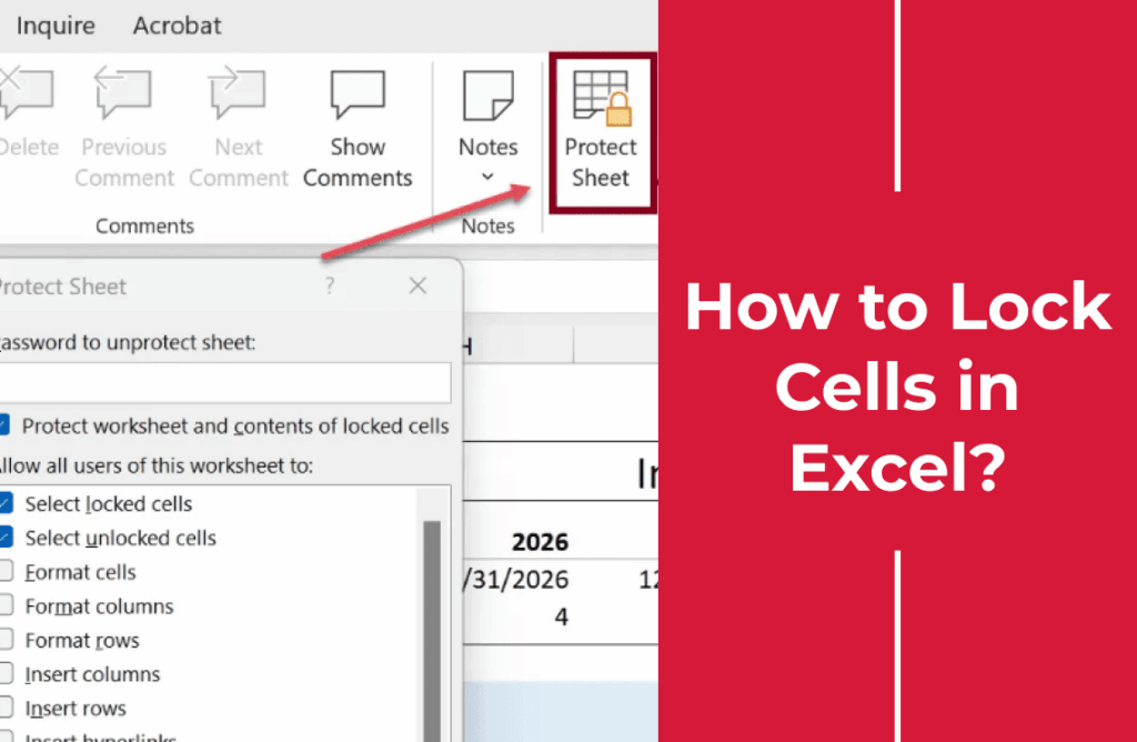
* **Go to the “Review” Tab:** In the Excel ribbon, click on the “Review” tab.
* **Click “Protect Sheet”:** In the “Protect” group, click on the “Protect Sheet” button. This will open the Protect Sheet dialog box.
* **Choose Protection Options:** In the Protect Sheet dialog box, you can choose which actions you want to allow users to perform on the worksheet. By default, the “Select locked cells” and “Select unlocked cells” options are checked. You can also allow users to format cells, insert rows, delete columns, and more. Be careful when selecting these options, as they can override the cell locking mechanism.
* **Set a Password (Optional):** If you want to prevent users from unprotecting the worksheet, enter a password in the “Password to unprotect sheet” box. **Important:** If you lose this password, you will not be able to unprotect the worksheet and unlock the cells. Consider storing the password in a safe place or using a password manager.
* **Click “OK”:** Click the “OK” button to protect the worksheet.
* **Re-enter Password (If Applicable):** If you entered a password, you will be prompted to re-enter it to confirm.
Congratulations! You have successfully locked an entire column in Excel. Now, when you try to edit any cell in the locked column, you will see a warning message indicating that the cell is protected. You can still edit cells in other columns that were not locked.
Advanced Techniques: Customizing Cell Locking
While locking an entire column is a common scenario, Excel offers more granular control over cell locking. Here are some advanced techniques for customizing cell locking:
Locking Specific Cells Within a Column
Sometimes, you may only want to lock certain cells within a column, while allowing users to edit other cells in the same column. Here’s how to do it:
* **Unlock the Entire Column:** First, unlock the entire column you want to work with, following the steps outlined in the previous section.
* **Select the Cells to Lock:** Select the specific cells you want to lock within the column. You can select multiple non-adjacent cells by holding down the `Ctrl` key (or `Cmd` key on a Mac) while clicking on each cell.
* **Open the Format Cells Dialog Box:** Right-click on the selected cells and choose “Format Cells…” from the context menu. Alternatively, use the keyboard shortcut `Ctrl + 1` (or `Cmd + 1` on a Mac).
* **Go to the Protection Tab:** In the Format Cells dialog box, click on the “Protection” tab.
* **Check the “Locked” Box:** Check the box next to “Locked”. This will lock only the selected cells.
* **Click “OK”:** Click the “OK” button to close the Format Cells dialog box.
* **Protect the Worksheet:** Protect the worksheet as described in Step 4 of the previous section.
Now, only the specific cells you selected will be locked, while the rest of the cells in the column will remain editable.
Using Formulas to Dynamically Lock Cells
In some cases, you may want to lock cells based on certain conditions. For example, you might want to lock a cell if it contains a specific value or if a certain date has passed. You can achieve this using conditional formatting and a bit of VBA code (Visual Basic for Applications).
**Note:** This technique requires some knowledge of VBA programming. If you’re not familiar with VBA, you may want to consult a VBA tutorial or seek help from an Excel expert.
Here’s a general outline of the steps involved:
1. **Create a Conditional Formatting Rule:** Use conditional formatting to highlight the cells you want to lock based on your criteria. For example, you can use a formula like `=A1=”Locked”` to highlight cells in column A that contain the word “Locked”.
2. **Write a VBA Macro:** Write a VBA macro that runs when the worksheet is changed. This macro will check the conditional formatting of each cell and lock or unlock it accordingly.
3. **Use the `Locked` Property:** In the VBA macro, use the `Locked` property of the `Range` object to lock or unlock the cells. For example, `Range(“A1”).Locked = True` will lock cell A1.
4. **Protect the Worksheet:** Protect the worksheet to activate the cell locking mechanism.
This technique allows you to dynamically lock cells based on changing conditions, providing a powerful way to control data entry and prevent unauthorized modifications.
Hiding Formulas to Protect Intellectual Property
In addition to locking cells, you may also want to hide the formulas behind certain cells to protect your intellectual property. This prevents users from seeing how you calculated your results, which can be particularly useful if you’re sharing your spreadsheet with external parties.
Here’s how to hide formulas:
* **Select the Cells with Formulas:** Select the cells containing the formulas you want to hide.
* **Open the Format Cells Dialog Box:** Right-click on the selected cells and choose “Format Cells…” from the context menu. Alternatively, use the keyboard shortcut `Ctrl + 1` (or `Cmd + 1` on a Mac).
* **Go to the Protection Tab:** In the Format Cells dialog box, click on the “Protection” tab.
* **Check the “Hidden” Box:** Check the box next to “Hidden”. This will hide the formulas in the selected cells when the worksheet is protected.
* **Click “OK”:** Click the “OK” button to close the Format Cells dialog box.
* **Protect the Worksheet:** Protect the worksheet as described in Step 4 of the previous section. Make sure the “Select locked cells” and “Select unlocked cells” options are checked.
Now, when you select a cell with a hidden formula, the formula will not be displayed in the formula bar. This provides an extra layer of protection for your intellectual property.
Troubleshooting Common Cell Locking Issues
Even with careful planning, you may encounter some common issues when locking cells in Excel. Here are some troubleshooting tips to help you resolve them:
* **Cells Still Editable After Protection:**
* **Cause:** The most common cause is that the cells were not locked before the worksheet was protected. Remember that all cells are unlocked by default, so you need to explicitly lock the cells you want to protect before enabling worksheet protection.
* **Solution:** Unprotect the worksheet, lock the desired cells, and then re-protect the worksheet.
* **Cannot Edit Unlocked Cells:**
* **Cause:** This can happen if you accidentally restricted the allowed actions in the Protect Sheet dialog box. For example, if you unchecked the “Select unlocked cells” option, users will not be able to select or edit any cells, even if they are unlocked.
* **Solution:** Unprotect the worksheet and check the protection options in the Protect Sheet dialog box. Make sure the “Select unlocked cells” option is checked.
* **Forgot the Password to Unprotect the Worksheet:**
* **Cause:** You forgot the password you set when protecting the worksheet.
* **Solution:** Unfortunately, there is no built-in way to recover a lost worksheet password in Excel. You may need to use a third-party password recovery tool, but be aware that these tools may not always work and can pose security risks. The best solution is to store your passwords in a safe place or use a password manager.
* **Formulas Not Hiding After Protection:**
* **Cause:** The “Hidden” option was not checked in the Format Cells dialog box before protecting the worksheet.
* **Solution:** Unprotect the worksheet, check the “Hidden” option for the cells with formulas, and then re-protect the worksheet.
* **Cell Locking Not Working as Expected with Shared Workbooks:**
* **Cause:** Shared workbooks have limited support for cell locking and protection. Some features may not work as expected.
* **Solution:** Consider using Excel’s co-authoring feature instead of shared workbooks. Co-authoring provides better support for cell locking and protection.
Best Practices for Cell Locking in Excel
To ensure that your cell locking strategy is effective and maintainable, follow these best practices:
* **Plan Your Protection Strategy:** Before locking any cells, carefully plan which cells need to be protected and which cells should remain editable. Consider the needs of all users who will be accessing the spreadsheet.
* **Document Your Protection Strategy:** Document your cell locking strategy, including which cells are locked, why they are locked, and any passwords used. This will help you and others understand and maintain the protection over time.
* **Use Descriptive Names for Locked Cells:** If you’re using formulas that refer to locked cells, use descriptive names for those cells. This will make your formulas easier to understand and maintain.
* **Provide Clear Instructions to Users:** Provide clear instructions to users on how to use the spreadsheet and which cells they are allowed to edit. This will help prevent accidental data alteration.
* **Test Your Protection Strategy:** After implementing your cell locking strategy, thoroughly test it to ensure that it works as expected. Try to edit locked cells and see if the protection is effective.
* **Regularly Review and Update Your Protection Strategy:** As your spreadsheet evolves, regularly review and update your cell locking strategy to ensure that it still meets your needs. You may need to lock or unlock different cells as your data and formulas change.
* **Use Strong Passwords:** If you’re using passwords to protect your worksheets, use strong passwords that are difficult to guess. A strong password should be at least 12 characters long and include a mix of uppercase and lowercase letters, numbers, and symbols. Avoid using personal information or common words in your passwords.
* **Store Passwords Securely:** Store your passwords in a safe place or use a password manager. Avoid writing passwords down on paper or storing them in plain text on your computer.
* **Consider Using Data Validation:** In addition to cell locking, consider using data validation to restrict the type of data that can be entered into certain cells. This can help prevent errors and maintain data integrity.
* **Use Excel’s Co-authoring Feature:** If you’re collaborating on a spreadsheet with multiple users, use Excel’s co-authoring feature instead of shared workbooks. Co-authoring provides better support for cell locking and protection, as well as real-time collaboration features.
Conclusion: Mastering Cell Locking for Excel Success
Locking cells in Excel columns is a simple yet powerful technique for protecting your data integrity and ensuring the accuracy of your spreadsheets. By understanding the basics of cell locking, following the step-by-step instructions in this guide, and implementing the best practices, you can confidently safeguard your work and prevent accidental or malicious data alteration.
Whether you’re a seasoned Excel user or just starting out, mastering cell locking is an essential skill for anyone who works with spreadsheets. So, take the time to learn these techniques and incorporate them into your workflow. Your data will thank you for it!
