Unlocking Motion’s Secrets: A Comprehensive Guide to Finding Acceleration, Position, and Time Graphs

Have you ever watched a car zoom by and wondered about the intricate dance of physics governing its motion? Or perhaps you’ve pondered how engineers design roller coasters that thrill us without sending us flying off the tracks? The key to understanding and predicting such movements lies in the relationship between acceleration, position, and time, often visualized through graphs. These graphs aren’t just squiggly lines; they’re powerful tools that reveal the hidden story of an object’s journey.

Why are Acceleration, Position, and Time Graphs Important?

Imagine trying to describe the trajectory of a baseball without using numbers or visuals. It would be a confusing mess! Acceleration, position, and time graphs provide a clear, concise, and mathematical way to represent motion. They allow us to:

• Visualize Motion: See how an object’s position, velocity, and acceleration change over time.
• Predict Future Motion: Use current data to estimate where an object will be and how fast it will be going at a later time.
• Analyze Complex Systems: Break down complicated movements into simpler, understandable components.
• Design and Optimize: Engineers use these graphs to design everything from cars and airplanes to robots and roller coasters.
• Diagnose Problems: Detect anomalies in motion, such as unexpected accelerations or decelerations.

In essence, these graphs are the language of motion. Mastering them unlocks a deeper understanding of the physical world around us.

Understanding the Basics: Position, Velocity, and Acceleration

Before diving into the graphs themselves, let’s refresh our understanding of the fundamental concepts they represent:

Position

Position refers to an object’s location in space at a particular moment in time. It’s usually measured relative to a reference point (origin). For example, a car might be 10 meters east of a traffic light, or a bird might be 50 meters above the ground. Position is a vector quantity, meaning it has both magnitude (distance) and direction.

Velocity

Velocity describes how quickly an object’s position is changing and in what direction. It’s the rate of change of position with respect to time. A car traveling at 60 miles per hour eastward has a velocity of 60 mph east. Velocity is also a vector quantity.

Acceleration

Acceleration, the star of our show, describes how quickly an object’s velocity is changing. It’s the rate of change of velocity with respect to time. A car speeding up from 0 to 60 mph in 5 seconds is accelerating. Like position and velocity, acceleration is a vector quantity.

The relationship between these three quantities is crucial. Velocity is the derivative of position with respect to time, and acceleration is the derivative of velocity with respect to time. Conversely, velocity is the integral of acceleration with respect to time, and position is the integral of velocity with respect to time. These calculus concepts form the mathematical backbone of motion analysis.

Creating and Interpreting Position-Time Graphs

A position-time graph plots an object’s position on the y-axis against time on the x-axis. This graph provides a visual representation of how an object’s location changes over time.

Key Features of a Position-Time Graph

• Slope: The slope of the line at any point on the graph represents the object’s instantaneous velocity at that time. A steeper slope indicates a higher velocity. A horizontal line indicates that the object is stationary (zero velocity).
• Curvature: The curvature of the graph indicates the object’s acceleration. A straight line implies constant velocity (zero acceleration). A curved line indicates that the velocity is changing (non-zero acceleration).
• Intercepts: The y-intercept represents the object’s initial position at time t=0. The x-intercept represents the time at which the object’s position is zero (i.e., it passes through the origin).

Interpreting Different Scenarios

• Constant Velocity: A straight line with a non-zero slope indicates constant velocity. The object is moving at a steady rate in a single direction.
• Increasing Velocity: A curve that gets steeper over time indicates increasing velocity (positive acceleration). The object is speeding up.
• Decreasing Velocity: A curve that gets less steep over time indicates decreasing velocity (negative acceleration or deceleration). The object is slowing down.
• Stationary Object: A horizontal line indicates that the object is not moving (zero velocity).
• Changing Direction: A change in the sign of the slope indicates a change in direction. For example, if the slope goes from positive to negative, the object has reversed its direction of motion.

Example: A Walk in the Park

Imagine a person walking in a park. Initially, they walk away from their starting point at a constant speed. Then, they slow down, stop for a moment to admire a flower, and finally walk back towards their starting point at a faster speed. The position-time graph would reflect this:

• A straight line with a positive slope (walking away at a constant speed).
• A curve that becomes less steep (slowing down).
• A horizontal line (stopped to admire the flower).
• A straight line with a negative slope (walking back towards the starting point). The negative slope would be steeper than the initial positive slope, indicating a faster speed.

Creating and Interpreting Velocity-Time Graphs

A velocity-time graph plots an object’s velocity on the y-axis against time on the x-axis. This graph provides a visual representation of how an object’s velocity changes over time.

Key Features of a Velocity-Time Graph

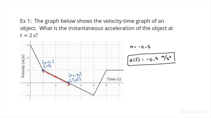
• Slope: The slope of the line at any point on the graph represents the object’s instantaneous acceleration at that time. A steeper slope indicates a larger acceleration. A horizontal line indicates constant velocity (zero acceleration).
• Area Under the Curve: The area under the curve between two points in time represents the object’s displacement (change in position) during that time interval.
• Intercepts: The y-intercept represents the object’s initial velocity at time t=0. The x-intercept represents the time at which the object’s velocity is zero.

Interpreting Different Scenarios

• Constant Velocity: A horizontal line indicates constant velocity (zero acceleration).
• Constant Acceleration: A straight line with a non-zero slope indicates constant acceleration. The velocity is changing at a steady rate.
• Increasing Acceleration: A curve that gets steeper over time indicates increasing acceleration. The rate at which the velocity is changing is increasing.
• Decreasing Acceleration: A curve that gets less steep over time indicates decreasing acceleration. The rate at which the velocity is changing is decreasing.
• Changing Direction: A change in the sign of the velocity indicates a change in direction. If the velocity goes from positive to negative, the object has reversed its direction of motion.

Example: A Car Accelerating

Imagine a car accelerating from rest to a certain speed. The velocity-time graph would show:

• A line starting at the origin (zero initial velocity).
• A straight line with a positive slope (constant acceleration). The slope represents the rate at which the car is speeding up.

If the car then maintains a constant speed, the graph would continue with a horizontal line.

Creating and Interpreting Acceleration-Time Graphs

An acceleration-time graph plots an object’s acceleration on the y-axis against time on the x-axis. This graph provides a visual representation of how an object’s acceleration changes over time.

Key Features of an Acceleration-Time Graph

• Area Under the Curve: The area under the curve between two points in time represents the object’s change in velocity during that time interval.
• Value: The y-value at any point on the graph represents the object’s instantaneous acceleration at that time.

Interpreting Different Scenarios

• Constant Acceleration: A horizontal line indicates constant acceleration.
• Zero Acceleration: A horizontal line at y=0 indicates zero acceleration (constant velocity or at rest).
• Increasing Acceleration: A line with a positive slope indicates increasing acceleration.
• Decreasing Acceleration: A line with a negative slope indicates decreasing acceleration.

Example: A Rocket Launch

Consider a rocket launch. Initially, the rocket experiences a large, relatively constant acceleration as its engines fire. As the rocket burns fuel, its mass decreases, and its acceleration may gradually increase. The acceleration-time graph would show:

• A horizontal line at a relatively high y-value (constant acceleration during the initial burn).
• A line with a slightly positive slope (gradually increasing acceleration as fuel is burned).

Finding Acceleration, Position, and Time Graphs: Different Approaches

Now that we understand the basics of these graphs, let’s explore different ways to find or generate them:

1. Experimental Data Collection

The most direct approach is to collect experimental data. This involves measuring an object’s position and time at various points during its motion. You can use a variety of tools for this purpose, such as:

• Motion Sensors: These sensors use technologies like ultrasound or infrared to measure an object’s distance and velocity. They can provide real-time data that can be directly plotted on graphs.
• Video Analysis: By recording an object’s motion and analyzing the video frame by frame, you can track its position over time. Software tools can automate this process and generate position-time data.
• Stopwatches and Measuring Tapes: For simpler experiments, you can manually measure an object’s position at specific time intervals using a stopwatch and measuring tape.

Once you have the position-time data, you can calculate the velocity and acceleration by finding the derivatives (slopes) of the position-time graph. Numerical methods can be used to approximate these derivatives if you don’t have a continuous function.

2. Mathematical Modeling

If you know the equations of motion governing an object’s movement, you can use mathematical modeling to generate the graphs. This involves:

• Defining the Equations of Motion: Identify the relevant physical laws and equations that describe the object’s motion. For example, for an object moving under constant acceleration, you can use the kinematic equations.
• Solving the Equations: Solve the equations to find expressions for position, velocity, and acceleration as functions of time.
• Plotting the Graphs: Use graphing software or programming tools to plot these functions and generate the position-time, velocity-time, and acceleration-time graphs.

This approach is particularly useful for analyzing idealized scenarios or for simulating the motion of complex systems.

3. Using Simulation Software

Several simulation software packages are available that can simulate the motion of objects and generate the corresponding graphs. These tools typically allow you to:

• Define the System: Specify the properties of the object, such as its mass, initial position, and initial velocity.
• Apply Forces: Define the forces acting on the object, such as gravity, friction, or applied forces.
• Run the Simulation: The software will simulate the object’s motion based on the defined parameters and forces.
• Visualize the Results: The software will generate position-time, velocity-time, and acceleration-time graphs, allowing you to analyze the object’s motion.

Examples of simulation software include:

• PhET Interactive Simulations: Offers a wide range of interactive physics simulations, including simulations of motion.
• MATLAB: A powerful programming environment that can be used for simulating and analyzing dynamic systems.
• SimScale: A cloud-based simulation platform that can be used for a variety of engineering simulations, including mechanical simulations.

4. From One Graph to Another: Differentiation and Integration

As mentioned earlier, the relationship between position, velocity, and acceleration is based on calculus. This means that you can derive one graph from another using differentiation and integration.

• From Position-Time to Velocity-Time: Find the slope of the position-time graph at various points in time. The slope at each point represents the instantaneous velocity at that time. Plot these velocities on a velocity-time graph.
• From Velocity-Time to Acceleration-Time: Find the slope of the velocity-time graph at various points in time. The slope at each point represents the instantaneous acceleration at that time. Plot these accelerations on an acceleration-time graph.
• From Acceleration-Time to Velocity-Time: Find the area under the acceleration-time graph between two points in time. The area represents the change in velocity during that time interval. Use this information to construct the velocity-time graph.
• From Velocity-Time to Position-Time: Find the area under the velocity-time graph between two points in time. The area represents the displacement (change in position) during that time interval. Use this information to construct the position-time graph.

Keep in mind that integration requires knowing the initial conditions (e.g., initial position or initial velocity) to determine the constant of integration.

Practical Applications of Acceleration, Position, and Time Graphs

The applications of these graphs are vast and span numerous fields:

• Engineering: Designing vehicles, bridges, and other structures that can withstand dynamic forces.
• Physics: Studying the motion of particles, planets, and other objects in the universe.
• Sports: Analyzing the performance of athletes and optimizing their training techniques.
• Robotics: Controlling the movement of robots and automating tasks.
• Medicine: Analyzing human movement and diagnosing medical conditions.
• Game Development: Creating realistic and engaging motion for characters and objects in video games.

For example, engineers use acceleration-time graphs to analyze the vibrations of bridges and buildings during earthquakes. This information helps them design structures that are more resistant to seismic activity. In sports, coaches use position-time and velocity-time graphs to analyze the running gait of athletes and identify areas for improvement.

Tips for Analyzing Acceleration, Position, and Time Graphs

Here are some helpful tips to keep in mind when analyzing these graphs:

• Pay attention to the units: Make sure you understand the units of measurement for position, velocity, acceleration, and time. This will help you interpret the graphs correctly.
• Look for patterns: Identify any patterns or trends in the graphs. Are there any periods of constant velocity, constant acceleration, or changing direction?
• Consider the context: Think about the physical situation that the graphs represent. What is the object doing? What forces are acting on it?
• Use calculus concepts: Remember the relationship between position, velocity, and acceleration. Use differentiation and integration to derive one graph from another.
• Practice, practice, practice: The more you practice analyzing these graphs, the better you will become at understanding them.

Common Mistakes to Avoid

Here are some common mistakes that students and beginners often make when working with these graphs:

• Confusing position, velocity, and acceleration: Remember that these are distinct concepts with different meanings and units.
• Misinterpreting the slope of the graph: The slope of a position-time graph represents velocity, while the slope of a velocity-time graph represents acceleration.
• Ignoring the area under the curve: The area under the velocity-time graph represents displacement, while the area under the acceleration-time graph represents change in velocity.
• Forgetting the initial conditions: When integrating to find position or velocity, remember to account for the initial conditions.
• Not paying attention to the units: Always make sure you are using consistent units throughout your calculations and analysis.

Conclusion: Mastering the Language of Motion

Acceleration, position, and time graphs are powerful tools for understanding and predicting motion. By mastering the concepts and techniques discussed in this guide, you can unlock a deeper appreciation of the physical world around you. Whether you’re an engineer designing a new vehicle, a physicist studying the motion of particles, or simply a curious individual seeking to understand how things move, these graphs provide a valuable framework for analysis and insight. So, embrace the challenge, practice your skills, and embark on a journey to unravel the secrets of motion!