

Unlocking the Secrets: How to Find the WiFi Password for Networks You’re Already Connected To
In today’s hyper-connected world, WiFi is practically a necessity. Whether you’re working from home, streaming your favorite shows, or just browsing the web, a stable WiFi connection is crucial. But what happens when you need to share your WiFi password with a guest, connect a new device, or simply can’t remember what cryptic combination of letters, numbers, and symbols you initially used? Don’t worry; you’re not alone! Forgetting your WiFi password is a common occurrence. The good news is that there are several straightforward methods to retrieve the password for networks you’re already connected to. This guide will walk you through those methods, step-by-step, across various operating systems and devices.
Why You Might Need to Find Your WiFi Password
Before diving into the how-to, let’s quickly consider why you might need to find your WiFi password in the first place:
- Sharing with Guests: Perhaps the most common scenario. Your friends, family, or visitors need internet access, and you don’t want to give them your primary network password.
- Connecting New Devices: Adding a new laptop, tablet, smart TV, or gaming console to your home network requires the WiFi password.
- Router Reset: If you’ve recently reset your router to factory settings, you might need to re-enter the WiFi password on all your devices.
- Security Audits: Occasionally, it’s wise to review your network security settings, including your password, to ensure it’s strong and hasn’t been compromised.
- Simply Forgot: Let’s face it; we all forget things. Passwords, in particular, can be easily misplaced or forgotten, especially if they’re complex and not frequently used.
Finding Your WiFi Password on Windows
Windows provides several methods to retrieve your WiFi password. Here are the most reliable approaches:
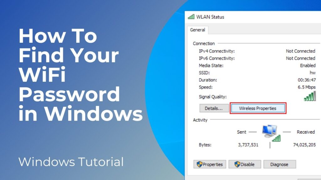
Method 1: Using the Control Panel
This is a classic and straightforward method that works on most Windows versions.
- Open the Control Panel: You can find it by searching for “Control Panel” in the Windows search bar.
- Navigate to Network and Sharing Center: Click on “Network and Internet,” then “Network and Sharing Center.”
- Click on Your WiFi Network Name: Find your active WiFi network connection and click on the link next to “Connections.” This will open the WiFi Status window.
- Wireless Properties: In the WiFi Status window, click on the “Wireless Properties” button.
- Security Tab: In the Wireless Properties window, go to the “Security” tab.
- Show Characters: Check the “Show characters” box. The WiFi password will now be displayed in the “Network security key” field.
This method is quick and easy, but it requires administrator privileges. If you don’t have admin rights, you’ll need to use another method.
Method 2: Using Command Prompt (CMD)
The Command Prompt is a powerful tool that allows you to interact with your system using text-based commands.
- Open Command Prompt as Administrator: Search for “cmd” in the Windows search bar, right-click on “Command Prompt,” and select “Run as administrator.” This is crucial; otherwise, the command won’t work.
- Enter the Command: Type the following command and press Enter:
netsh wlan show profile name="Your WiFi Network Name" key=clearReplace “Your WiFi Network Name” with the actual name of your WiFi network (SSID). Make sure to enclose the network name in quotation marks if it contains spaces.
- Find the Password: Look for the “Key Content” field in the output. This field contains your WiFi password.
This method is slightly more technical than the Control Panel method, but it’s still relatively easy to follow. Again, administrator privileges are required.
Method 3: Using PowerShell
PowerShell is a more advanced command-line shell and scripting language that’s also available on Windows.
- Open PowerShell as Administrator: Search for “PowerShell” in the Windows search bar, right-click on “Windows PowerShell,” and select “Run as administrator.”
- Enter the Command: Type the following command and press Enter:
(netsh wlan show profile name="Your WiFi Network Name" key=clear).split("n") | findstr "Key Content"Replace “Your WiFi Network Name” with the actual name of your WiFi network.
- Find the Password: The output will display the “Key Content” field, which contains your WiFi password.
PowerShell offers a slightly more concise way to retrieve the password compared to Command Prompt, but the principle remains the same. Administrator privileges are still necessary.
Finding Your WiFi Password on macOS
macOS offers a different set of tools for managing WiFi passwords. Here’s how to find your password on a Mac:
Using Keychain Access
Keychain Access is a built-in macOS utility that securely stores your passwords and other sensitive information.
- Open Keychain Access: You can find it by searching for “Keychain Access” in Spotlight (Cmd + Space). It’s located in the /Applications/Utilities/ folder.
- Search for Your WiFi Network: In the Keychain Access window, search for the name of your WiFi network (SSID) in the search bar.
- Double-Click on the Network Name: This will open a window with details about the WiFi network.
- Show Password: Check the “Show Password” box. You’ll be prompted to enter your administrator password to authenticate.
- Enter Your Administrator Password: Enter your macOS administrator password. The WiFi password will now be displayed.
Keychain Access is the primary method for managing passwords on macOS. It’s a secure and convenient way to store and retrieve your WiFi password.
Finding Your WiFi Password on Android
The method for finding your WiFi password on Android varies slightly depending on the Android version and manufacturer. However, here are the most common approaches:
Method 1: Using the WiFi Settings (Android 10 and Later)
Android 10 and later versions offer a built-in feature to share WiFi passwords via a QR code or by displaying the password directly.
- Open Settings: Go to your phone’s Settings app.
- Navigate to WiFi: Tap on “WiFi.”
- Select Your Connected Network: Tap on the name of your connected WiFi network.
- Share or QR Code: Look for a “Share” button or a QR code icon. Tapping on “Share” might require you to authenticate with your fingerprint, PIN, or password.
- View the Password: Depending on your device, the password might be displayed directly, or you might need to scan the QR code using another device to reveal the password.
This method is the easiest and most straightforward on newer Android devices.
Method 2: Using a Rooted Device (All Android Versions)
If your Android device is rooted, you can access the WiFi password file directly.
Warning: Rooting your device can void your warranty and potentially brick your device if not done correctly. Proceed with caution and at your own risk.
- Install a Root File Explorer: You’ll need a file explorer that supports root access, such as Solid Explorer or Root Explorer.
- Navigate to the WiFi Configuration File: Open the file explorer and navigate to the following directory:
/data/misc/wifi/wpa_supplicant.conf - Open the File: Open the
wpa_supplicant.conffile with a text editor. - Find Your Network: Look for your WiFi network’s SSID within the file. The password (PSK) will be listed next to it.
This method requires a rooted device and a file explorer with root access. It provides direct access to the WiFi configuration file, allowing you to view all stored WiFi passwords.
Finding Your WiFi Password on iOS (iPhone/iPad)
Unfortunately, iOS doesn’t provide a built-in way to directly view the WiFi password for networks you’re connected to, without the use of third-party apps or workarounds. However, there are a few options:
Method 1: Using iCloud Keychain (If Synced with a Mac)
If you’ve synced your iCloud Keychain with a Mac, you can use the Keychain Access app on your Mac to view the WiFi password, as described in the macOS section above. The password will be synced across your devices.
Method 2: Using Third-Party Apps (Requires Jailbreaking)
Some third-party apps claim to be able to retrieve WiFi passwords on iOS, but these apps often require jailbreaking your device. Jailbreaking voids your warranty and can expose your device to security risks.
Warning: Jailbreaking your iOS device is not recommended unless you are an experienced user and understand the risks involved.
Method 3: Router Access
The most reliable method for finding your WiFi password when you can’t directly access it on your iOS device is to log in to your router’s administration panel. This method is detailed in a section below.
Finding Your WiFi Password Through Your Router
Accessing your router’s administration panel is a universal method that works regardless of your operating system or device. This method requires you to know your router’s IP address, username, and password.
Step 1: Find Your Router’s IP Address
Your router’s IP address is the gateway through which your devices connect to the internet. Here’s how to find it on different operating systems:
- Windows: Open Command Prompt (cmd) and type
ipconfig. Look for the “Default Gateway” address. - macOS: Open Terminal and type
netstat -nr | grep default. The IP address next to “default” is your router’s IP. - Android: Go to Settings > WiFi, tap on your connected network, and look for the “Gateway” address.
- iOS: Go to Settings > WiFi, tap on your connected network, and look for the “Router” address.
Step 2: Access Your Router’s Administration Panel
- Open a Web Browser: Open any web browser on your computer or mobile device.
- Enter the Router’s IP Address: Type your router’s IP address into the address bar and press Enter.
- Login: You’ll be prompted to enter your router’s username and password. If you haven’t changed them, the default credentials are often printed on a sticker on the router itself. Common default usernames are “admin” or “user,” and common default passwords are “admin,” “password,” or a blank field. If you’ve changed the credentials and forgotten them, you may need to reset your router to factory settings (which will erase all your custom settings).
Step 3: Find the WiFi Password
The location of the WiFi password within the router’s administration panel varies depending on the router’s manufacturer and model. However, it’s typically found in one of the following sections:
- Wireless Settings: Look for a section labeled “Wireless,” “WiFi,” or “Wireless Security.”
- Security Settings: The password might be located under “Security Settings” or “Wireless Security.”
- Basic Settings: In some cases, the password is displayed in the “Basic Settings” or “Quick Setup” section.
Once you’ve found the correct section, look for a field labeled “Password,” “Passphrase,” “Security Key,” or “PSK.” The WiFi password will be displayed in this field.
Important Security Considerations
While retrieving your WiFi password is often necessary, it’s also important to consider the security implications:
- Strong Passwords: Use strong, complex passwords that are difficult to guess. A strong password should be at least 12 characters long and include a combination of uppercase and lowercase letters, numbers, and symbols.
- Change Default Credentials: Always change the default username and password for your router’s administration panel. Default credentials are a security risk because they are publicly known.
- WPA3 Encryption: If your router supports it, use WPA3 encryption. WPA3 is the latest and most secure WiFi encryption protocol.
- Guest Network: Create a guest network for visitors. This allows them to access the internet without giving them access to your primary network and sensitive data.
- Regular Updates: Keep your router’s firmware up to date. Firmware updates often include security patches that protect your network from vulnerabilities.
- Monitor Connected Devices: Regularly review the list of devices connected to your network to ensure that only authorized devices are connected.
Troubleshooting Common Issues
Sometimes, you might encounter issues while trying to retrieve your WiFi password. Here are some common problems and their solutions:
- Incorrect Router IP Address: Make sure you’re using the correct router IP address. Double-check the IP address using the methods described above.
- Forgotten Router Credentials: If you’ve forgotten your router’s username and password, you may need to reset your router to factory settings. This will erase all your custom settings, so be sure to back them up if possible.
- Administrator Privileges Required: Some methods, such as using Command Prompt or PowerShell on Windows, require administrator privileges. Make sure you’re running the command prompt or PowerShell as an administrator.
- Incorrect Network Name: When using the Command Prompt or PowerShell, make sure you’re using the correct network name (SSID). The network name is case-sensitive.
- Keychain Access Issues: If you’re having trouble accessing Keychain Access on macOS, try restarting your Mac or repairing the keychain.
Conclusion
Finding your WiFi password when you’ve forgotten it doesn’t have to be a daunting task. Whether you’re using Windows, macOS, Android, or iOS, there are several methods available to retrieve your password. By following the steps outlined in this guide, you can easily find your WiFi password and share it with guests, connect new devices, or simply refresh your memory. Remember to prioritize security by using strong passwords, changing default credentials, and keeping your router’s firmware up to date. With a little effort, you can ensure that your WiFi network is both accessible and secure.
