

Introduction: Why Freeze Columns in Excel?
Excel, the ubiquitous spreadsheet software, is a powerhouse for data analysis, organization, and reporting. Whether you’re managing financial statements, tracking sales figures, or organizing customer data, Excel provides the tools you need to get the job done. However, as your spreadsheets grow in size and complexity, navigating through them can become a challenge. This is where the ability to freeze columns comes in handy. Freezing columns (or rows, for that matter) allows you to keep specific parts of your worksheet visible while scrolling through the rest of the data. This is incredibly useful when you need to compare data points across a large dataset or keep track of key identifiers as you move horizontally or vertically.
Imagine you have a spreadsheet with hundreds of columns, each representing a different month’s sales data. The first few columns contain customer names, product categories, and other essential information. Without freezing these columns, you would constantly have to scroll back to the beginning to remember which customer or product each data point refers to. This not only wastes time but also increases the risk of errors. By freezing the customer name and product category columns, you can keep them visible at all times, making it much easier to analyze and compare the sales data for each month.
This comprehensive guide will walk you through the various methods of freezing columns in Excel, providing step-by-step instructions and practical examples. We’ll cover everything from freezing a single column to freezing multiple columns and even freezing columns and rows simultaneously. Whether you’re a beginner or an experienced Excel user, you’ll find valuable tips and tricks to enhance your productivity and streamline your workflow.
Understanding the Freeze Panes Feature
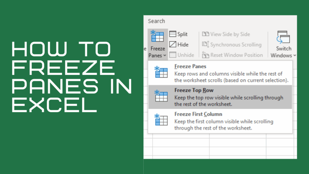
The core functionality that enables you to freeze columns in Excel is the “Freeze Panes” feature. This feature allows you to lock specific rows and columns in place, ensuring they remain visible as you scroll through the rest of your worksheet. The Freeze Panes feature is located in the “View” tab of the Excel ribbon, in the “Window” group. It offers three primary options:
- Freeze Panes: This option freezes rows above and columns to the left of the active cell.
- Freeze Top Row: This option freezes the first row of the worksheet.
- Freeze First Column: This option freezes the first column of the worksheet.
Understanding how these options work is crucial for effectively freezing columns in Excel. The “Freeze Panes” option is the most versatile, as it allows you to freeze any combination of rows and columns based on the position of the active cell. The “Freeze Top Row” and “Freeze First Column” options are simpler and more straightforward, but they are limited to freezing only the first row or column, respectively.
Step-by-Step Guide: Freezing the First Column
Freezing the first column is perhaps the simplest and most common use case for the Freeze Panes feature. It’s particularly useful when you have a list of items in the first column (e.g., customer names, product codes, employee IDs) and want to keep them visible as you scroll through the other columns. Here’s how to do it:
- Open your Excel spreadsheet: Launch Excel and open the spreadsheet you want to work with.
- Navigate to the “View” tab: Click on the “View” tab in the Excel ribbon.
- Click on “Freeze Panes”: In the “Window” group, click on the “Freeze Panes” dropdown menu.
- Select “Freeze First Column”: Choose the “Freeze First Column” option from the dropdown menu.
That’s it! The first column of your spreadsheet is now frozen. You can scroll horizontally through the other columns, and the first column will remain visible at all times. To unfreeze the first column, simply repeat the steps above and select “Unfreeze Panes” from the dropdown menu.
Freezing Multiple Columns: A Detailed Walkthrough
In many cases, you may need to freeze more than just the first column. For example, you might want to freeze the first two or three columns to keep multiple identifiers visible. Here’s how to freeze multiple columns in Excel:
- Select the column to the right of the columns you want to freeze: This is a crucial step. Excel freezes all columns to the left of the selected column. For example, if you want to freeze the first two columns (A and B), you need to select column C.
- Navigate to the “View” tab: Click on the “View” tab in the Excel ribbon.
- Click on “Freeze Panes”: In the “Window” group, click on the “Freeze Panes” dropdown menu.
- Select “Freeze Panes”: Choose the “Freeze Panes” option from the dropdown menu.
Now, all columns to the left of the selected column (in this case, columns A and B) are frozen. You can scroll horizontally, and these columns will remain visible. To unfreeze the columns, repeat the steps and select “Unfreeze Panes” from the dropdown menu.
Example: Let’s say you have a spreadsheet with customer data, including customer ID, name, and address in columns A, B, and C, respectively. You want to freeze these three columns so that you can easily identify each customer as you scroll through their purchase history in the subsequent columns. To do this, you would select column D, navigate to the “View” tab, click on “Freeze Panes,” and select “Freeze Panes.” Columns A, B, and C will now be frozen.
Freezing Columns and Rows Simultaneously
Sometimes, you may need to freeze both columns and rows at the same time. This is particularly useful when you have a large dataset with both row and column headers that you want to keep visible. Here’s how to freeze both columns and rows:
- Select the cell below the rows and to the right of the columns you want to freeze: This is the most important step. Excel freezes all rows above and all columns to the left of the selected cell. For example, if you want to freeze the first row (row 1) and the first column (column A), you need to select cell B2.
- Navigate to the “View” tab: Click on the “View” tab in the Excel ribbon.
- Click on “Freeze Panes”: In the “Window” group, click on the “Freeze Panes” dropdown menu.
- Select “Freeze Panes”: Choose the “Freeze Panes” option from the dropdown menu.
Now, all rows above and all columns to the left of the selected cell are frozen. You can scroll horizontally and vertically, and the frozen rows and columns will remain visible. To unfreeze the rows and columns, repeat the steps and select “Unfreeze Panes” from the dropdown menu.
Example: Imagine you have a spreadsheet with sales data for different products across different months. The first row contains the month names (e.g., January, February, March), and the first column contains the product names (e.g., Product A, Product B, Product C). You want to freeze both the row of month names and the column of product names so that you can easily see which product and month each data point refers to. To do this, you would select cell B2, navigate to the “View” tab, click on “Freeze Panes,” and select “Freeze Panes.” The first row and the first column will now be frozen.
Troubleshooting Common Issues
While freezing columns in Excel is generally straightforward, you may encounter some issues from time to time. Here are some common problems and their solutions:
- Columns are not freezing as expected: This is often due to selecting the wrong cell or column before freezing the panes. Double-check that you have selected the correct cell or column based on which rows and columns you want to freeze. Remember, Excel freezes rows above and columns to the left of the selected cell or column.
- The “Freeze Panes” option is grayed out: This can happen if the worksheet is protected or if you are in a shared workbook with certain restrictions. Check if the worksheet is protected and, if so, unprotect it. If you are in a shared workbook, contact the workbook owner to see if there are any restrictions preventing you from using the Freeze Panes feature.
- The frozen columns disappear when printing: By default, Excel does not print frozen panes. To print the frozen columns, you need to adjust the print settings. Go to the “Page Layout” tab, click on “Print Titles,” and specify the rows and columns you want to repeat on each page.
Advanced Tips and Tricks
Here are some advanced tips and tricks to help you get the most out of the Freeze Panes feature:
- Using Freeze Panes with Split Windows: You can combine the Freeze Panes feature with split windows to create even more flexible views of your data. Split windows allow you to divide your worksheet into multiple panes, each of which can be scrolled independently. By freezing columns in one pane and scrolling through the other, you can easily compare different parts of your data side-by-side.
- Freezing Columns in Excel Online: The Freeze Panes feature is also available in Excel Online, the web-based version of Excel. The steps for freezing columns in Excel Online are similar to those in the desktop version. However, there may be some limitations in terms of functionality and performance.
- Using VBA to Freeze Columns: For advanced users, you can use Visual Basic for Applications (VBA) to automate the process of freezing columns. This can be useful if you need to freeze columns based on certain conditions or if you want to create a custom button or macro to freeze columns with a single click.
Practical Examples and Use Cases
To further illustrate the power and versatility of the Freeze Panes feature, let’s look at some practical examples and use cases:
- Financial Reporting: In financial reporting, you often need to compare financial data across different periods (e.g., months, quarters, years). By freezing the row of account names and the column of period names, you can easily analyze the financial performance of each account over time.
- Sales Tracking: In sales tracking, you may want to keep track of customer names, product categories, and sales representatives while scrolling through the sales data for each month. By freezing the relevant columns, you can easily identify the customer, product, and sales representative associated with each sale.
- Project Management: In project management, you can use Excel to track tasks, deadlines, and resources. By freezing the column of task names, you can easily see the status of each task as you scroll through the project timeline.
- Inventory Management: In inventory management, you can use Excel to track the quantity of each item in stock. By freezing the column of item names, you can easily see the inventory level of each item as you scroll through the warehouse locations.
Conclusion: Mastering Excel with Freeze Columns
Freezing columns in Excel is a simple yet powerful technique that can significantly enhance your productivity and streamline your workflow. By keeping key identifiers visible as you scroll through your data, you can reduce errors, save time, and gain deeper insights. Whether you’re a beginner or an experienced Excel user, mastering the Freeze Panes feature is an essential skill for anyone who works with spreadsheets on a regular basis. From freezing a single column to freezing multiple columns and rows simultaneously, this guide has provided you with the knowledge and tools you need to effectively freeze columns in Excel and take your spreadsheet skills to the next level. So go ahead, experiment with the Freeze Panes feature, and discover how it can transform the way you work with Excel.
Embrace the power of organized data, and let Excel’s Freeze Panes be your trusty companion in navigating the vast landscapes of your spreadsheets. Happy Excelling!
