

Feeling Overwhelmed? Your Guide to Leaving a Discord Server
Discord, the bustling hub of online communities, gaming squads, and friendly chats, can sometimes feel… a bit much. Maybe the server you joined months ago is now overflowing with notifications, or perhaps the community vibe just isn’t your cup of tea anymore. Whatever the reason, knowing how to quickly leave a Discord server is a valuable skill. This comprehensive guide will walk you through the process, explain why you might want to leave in the first place, and offer some helpful tips for managing your Discord experience.
Why Leave a Discord Server? More Reasons Than You Think
Before we dive into the ‘how,’ let’s explore the ‘why.’ Leaving a Discord server isn’t always a sign of negativity. Sometimes, it’s simply a matter of managing your online space and priorities. Here are a few common reasons people choose to bid farewell to a server:
- Notification Overload: Constant pings and message alerts can be distracting and even anxiety-inducing. If a server is buzzing non-stop, leaving might be the best way to regain your peace of mind.
- Irrelevant Content: Interests change! A server that once aligned with your hobbies might now be focused on topics you no longer care about.
- Toxic Environment: Unfortunately, not all online communities are created equal. If you encounter harassment, negativity, or generally unpleasant behavior, leaving is a perfectly valid response. Your mental health comes first.
- Lack of Engagement: Maybe you joined a server with high hopes but haven’t found yourself actively participating. If you’re just lurking and not getting any value, it might be time to move on.
- Time Management: Let’s face it, Discord can be a time sink. Leaving servers that aren’t essential can free up your schedule for other activities.
- Server Inactivity: Sometimes, servers simply die. If the community is no longer active and conversations are few and far between, there’s little point in sticking around.
- New Interests: As you explore new hobbies and passions, you might find yourself gravitating towards different online communities. Leaving older servers makes room for new connections.
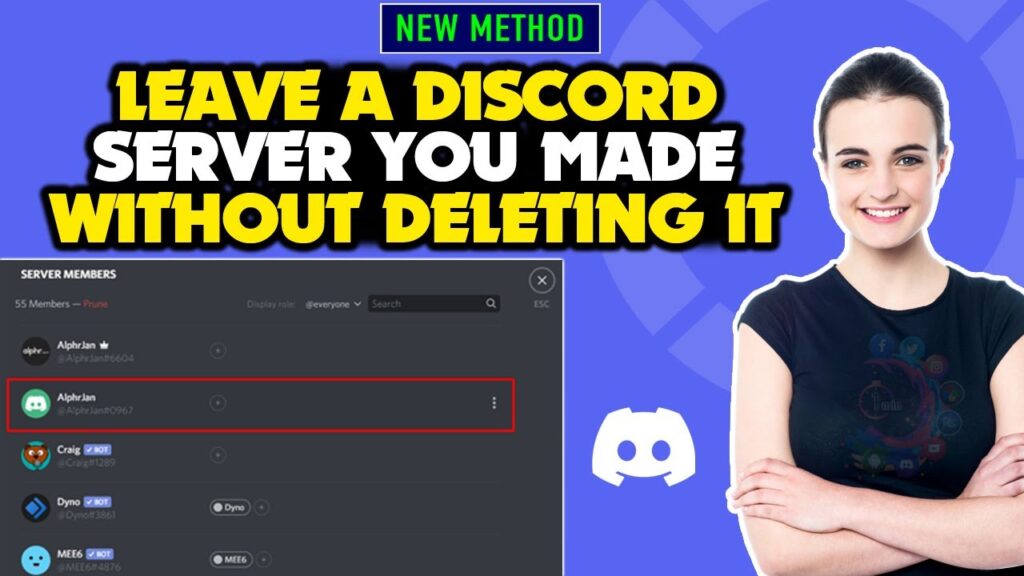
The Quick and Easy Guide: How to Leave a Discord Server
Ready to make your exit? Here’s how to leave a Discord server in just a few simple steps. The process is virtually identical across the desktop app, the web browser version, and the mobile app.
Leaving a Server on Desktop (App or Browser)
- Locate the Server Icon: On the left-hand side of your Discord window, you’ll see a vertical list of server icons. Find the icon for the server you want to leave.
- Right-Click the Icon: Right-click on the server icon. This will open a context menu.
- Select “Leave Server”: In the context menu, you’ll see an option that says “Leave Server.” Click on it.
- Confirmation: A pop-up window will appear, asking you to confirm your decision. Click the “Leave Server” button to finalize your departure.
Leaving a Server on Mobile (iOS or Android)
- Open the Discord App: Launch the Discord app on your smartphone or tablet.
- Access the Server List: Tap the three horizontal lines (the “hamburger” menu) in the top-left corner of the screen to open the server list.
- Long-Press the Server Icon: Find the icon for the server you want to leave and long-press (tap and hold) on it.
- Select “Leave Server”: A menu will appear. Tap on the “Leave Server” option.
- Confirmation: A confirmation message will pop up. Tap “Yes” or “Leave” to confirm that you want to leave the server.
Before You Go: A Few Things to Consider
Leaving a server is usually a straightforward decision, but here are a few things to keep in mind before you click that final “Leave” button:
- Saying Goodbye (Optional): If you’ve formed close relationships with people on the server, you might want to send a quick farewell message before leaving. This is entirely optional, but it’s a nice gesture, especially in smaller communities.
- Direct Messages: Leaving a server doesn’t automatically remove your direct message conversations with other members. You’ll still be able to access those messages unless the other person blocks you.
- Rejoining: In most cases, you can rejoin a server if you change your mind later. However, some servers have invite restrictions or require administrator approval for re-entry.
- Alternative: Muting and Notification Settings: Before leaving, consider if muting the server or adjusting notification settings might solve your problem. You can mute an entire server or customize notifications for specific channels. This allows you to stay connected without being overwhelmed.
Muting vs. Leaving: Which is Right for You?
Sometimes, leaving a server feels like a drastic measure. Discord offers alternative options that might be a better fit, particularly if you’re on the fence about leaving entirely. Muting a server is a great way to reduce the noise without cutting ties completely.
How to Mute a Discord Server
The process for muting a server is similar to leaving, but instead of selecting “Leave Server,” you’ll choose the mute option.
On Desktop:
- Right-click the server icon.
- Hover over “Mute Server.”
- Choose a mute duration (15 minutes, 1 hour, 8 hours, 24 hours, or Until I turn it back on).
On Mobile:
- Long-press the server icon.
- Tap “Mute.”
- Choose a mute duration.
Customizing Notification Settings
Discord’s notification settings are incredibly granular. You can customize notifications for individual channels or even specific users. This allows you to stay informed about the conversations that matter most to you while filtering out the noise.
To access notification settings:
- Right-click the server icon (on desktop) or long-press it (on mobile).
- Select “Notification Settings.”
- From here, you can choose to receive all messages, only mentions, or nothing at all. You can also customize notifications for individual channels within the server.
Server Management Tips for a Better Discord Experience
Beyond leaving or muting servers, there are several other strategies you can use to manage your Discord experience and create a more enjoyable online environment.
- Organize Your Server List: If you’re a member of many servers, consider organizing them into folders. This can make it easier to find the servers you’re looking for and reduce clutter.
- Utilize Discord’s Search Function: Need to find a specific message or piece of information? Discord’s search function is your friend. Use keywords to quickly locate what you’re looking for.
- Manage Your Friend List: Keep your friend list up-to-date by removing inactive or unwanted contacts. This can help you stay focused on the people you genuinely want to connect with.
- Set Clear Boundaries: It’s okay to disconnect from Discord and prioritize your offline life. Don’t feel pressured to be constantly available or responsive.
- Report Problematic Behavior: If you encounter harassment, abuse, or other violations of Discord’s terms of service, report it to the platform’s moderation team.
- Create Your Own Server: If you’re not finding the communities you’re looking for, consider creating your own server. This gives you complete control over the environment and allows you to build a community that aligns with your values.
The Psychology of Leaving: It’s Okay to Disconnect
In today’s hyper-connected world, it’s easy to feel obligated to stay engaged in online communities, even when they’re no longer serving your needs. However, it’s important to remember that disconnecting is a healthy and necessary part of maintaining your mental well-being. Leaving a Discord server isn’t a failure; it’s a conscious choice to prioritize your time, energy, and emotional health.
Think of your online presence as a garden. You need to prune away the elements that are no longer thriving to make room for new growth. Leaving a server that’s draining your energy allows you to cultivate connections that are more meaningful and fulfilling.
When to Consider a More Permanent Solution: Deleting Your Discord Account
While leaving a server is a simple and reversible action, there might be times when you need a more permanent solution. If you’re completely done with Discord and want to remove your presence from the platform entirely, you can delete your account.
Important Note: Deleting your Discord account is a permanent action. All your data, including your messages, friends, and server memberships, will be permanently deleted. There is no way to recover your account once it’s been deleted.
How to Delete Your Discord Account
- Log in to your Discord account: Access Discord through the desktop app or web browser. You cannot delete your account from the mobile app.
- Go to User Settings: Click the gear icon next to your username in the bottom-left corner of the screen.
- Select “My Account”: In the left-hand menu, click on “My Account.”
- Scroll Down and Click “Delete Account”: At the bottom of the “My Account” page, you’ll see a button that says “Delete Account.” Click on it.
- Two-Factor Authentication (if enabled): If you have two-factor authentication enabled, you’ll need to enter your authentication code.
- Enter Your Password: You’ll be prompted to enter your password to confirm that you want to delete your account.
- Final Confirmation: Click the “Delete Account” button to finalize the deletion process.
Disabling Your Account: As an alternative to deleting your account, you can also choose to disable it. Disabling your account makes it invisible to other users, but it allows you to reactivate it later if you change your mind.
In Conclusion: Take Control of Your Discord Experience
Discord is a powerful platform for connecting with others and building online communities. However, it’s important to remember that you’re in control of your own experience. Knowing how to quickly leave a Discord server, manage your notification settings, and set clear boundaries are essential skills for maintaining a healthy and enjoyable online presence. Don’t be afraid to disconnect when you need to, and always prioritize your mental well-being.
So, the next time you find yourself feeling overwhelmed by a particular server, remember this guide. A quick click or tap is all it takes to reclaim your peace of mind and curate a Discord experience that truly serves your needs.
