How to Pin Rows in Excel: A Comprehensive Guide
Freezing panes in Excel is a crucial skill for anyone working with large spreadsheets. This guide will walk you through how to pin rows (and columns!) in Excel, significantly improving your workflow and making navigating extensive datasets a breeze. We'll cover various methods and scenarios, ensuring you become a pro at managing your Excel spreadsheets.
Why Pin Rows in Excel?
Working with massive spreadsheets can be overwhelming. Scrolling through hundreds or thousands of rows to find specific data points is time-consuming and frustrating. Pinning, or freezing, rows keeps important header rows or summary rows visible at the top of your spreadsheet, no matter how far you scroll down. This dramatically increases efficiency and reduces errors.
Key Benefits of Pinning Rows:
- Improved Data Visibility: Keep critical header information readily accessible while exploring the dataset.
- Enhanced Accuracy: Reduce errors by always having context for the data you're viewing.
- Increased Productivity: Navigate large spreadsheets much faster, saving you valuable time.
How to Pin Rows (and Columns!) in Excel: Step-by-Step Guide
There are several ways to freeze rows in Excel, depending on your version and preferences. Here's a breakdown of the most common methods:
Method 1: Using the "Freeze Panes" Feature
This is the most straightforward method and works across most Excel versions:
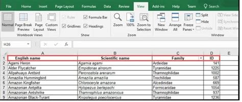
- Select the cell: Click on the cell below the row you want to freeze. For example, if you want to freeze the first row, click on cell A2. If you want to freeze the first two rows, click on cell A3.
- Access Freeze Panes: Go to the "View" tab in the Excel ribbon.
- Click "Freeze Panes": This will freeze all rows above and columns to the left of the selected cell.
Now, as you scroll down or to the right, the rows and columns you've frozen will remain visible.
Method 2: Freezing Specific Rows and Columns Simultaneously
You can also freeze specific rows and columns at the same time:
- Select the cell: Click the cell below the row and to the right of the column you want to freeze. For example, to freeze the first row and the first column, select cell B2.
- Access Freeze Panes: Go to the "View" tab and click "Freeze Panes".
This method allows you to keep both header rows and columns visible, regardless of scrolling.
Method 3: Unfreezing Panes
To unfreeze your rows and columns, simply follow these steps:
- Go to the "View" tab.
- Click "Freeze Panes".
- Select "Unfreeze Panes". This will restore the spreadsheet to its unfrozen state.
Troubleshooting and Tips
- Accidental Freezing: If you accidentally freeze the wrong rows or columns, simply unfreeze the panes and repeat the process.
- Multiple Freezes: You can only have one active freeze panes setting at a time. Unfreeze before applying a new freeze.
- Large Datasets: For extremely large datasets, consider using Excel's filtering and sorting capabilities in conjunction with frozen panes for optimal navigation.
Conclusion
Mastering the art of pinning rows in Excel is a game-changer for anyone working with large spreadsheets. By following these simple steps, you can significantly improve your productivity, accuracy, and overall Excel experience. Remember to experiment with different methods to find the best workflow for your specific needs. Now go forth and conquer those massive spreadsheets!
