

Introduction: Streamlining Data Management with Checkboxes in Excel
Microsoft Excel, a ubiquitous tool in the world of data management, offers a plethora of features to organize, analyze, and present information. While many users are familiar with basic functionalities like formulas and charts, Excel also provides options for interactive elements that can significantly enhance usability. One such element is the checkbox. Adding checkboxes to each row in Excel can transform static spreadsheets into dynamic tools for tracking progress, managing tasks, and conducting surveys. This comprehensive guide will walk you through various methods to seamlessly integrate checkboxes into your Excel worksheets, making your data management tasks more efficient and intuitive.
Imagine you’re managing a project with multiple tasks, each assigned to a different team member. Instead of manually updating the status of each task, you can add a checkbox next to each one. Team members can simply check the box when they complete their task, providing an instant visual update of the project’s progress. Or, consider a survey where respondents can select multiple options from a list. Checkboxes allow them to easily indicate their choices, simplifying the data collection process. The possibilities are endless, and the impact on productivity can be substantial.
This guide will cover everything from enabling the Developer tab (a prerequisite for many checkbox methods) to using the legacy Forms controls and the more modern ActiveX controls. We’ll also explore alternative approaches, such as using symbols or data validation, to achieve a similar effect. Whether you’re a beginner or an experienced Excel user, you’ll find practical tips and step-by-step instructions to help you master the art of adding checkboxes to your spreadsheets. Let’s dive in and unlock the full potential of your Excel data management!
Enabling the Developer Tab: Your Gateway to Advanced Features
Before we can start adding checkboxes, we need to ensure that the Developer tab is visible in your Excel ribbon. This tab provides access to advanced features, including the controls we’ll be using. By default, the Developer tab is hidden, but enabling it is a simple process.
Step-by-Step Guide to Enabling the Developer Tab
- Open Excel Options: Click on the “File” tab in the top-left corner of the Excel window.
- Navigate to Options: In the backstage view, click on “Options” at the bottom of the left-hand menu.
- Customize the Ribbon: In the Excel Options dialog box, select “Customize Ribbon” from the left-hand menu.
- Check the Developer Box: On the right-hand side, under the “Customize the Ribbon” section, you’ll see a list of main tabs. Find the “Developer” checkbox and tick it.
- Apply Changes: Click “OK” to close the Excel Options dialog box.
Once you’ve completed these steps, the Developer tab should now be visible in your Excel ribbon. You’re now ready to explore the world of controls and start adding checkboxes to your worksheets.
Method 1: Using Form Controls Checkboxes
Form Controls are a classic way to add interactive elements to your Excel spreadsheets. They are relatively simple to use and provide basic checkbox functionality. Here’s how to add a Form Control checkbox:
Step-by-Step Guide to Adding Form Control Checkboxes
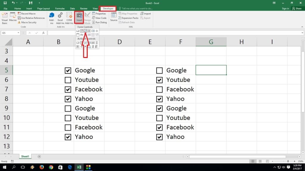
- Select the Developer Tab: Click on the “Developer” tab in the Excel ribbon.
- Insert a Checkbox: In the “Controls” group, click on “Insert” and then select the checkbox icon under the “Form Controls” section.
- Draw the Checkbox: Click and drag on your worksheet to draw the checkbox. You can resize and reposition it as needed.
- Edit the Text: By default, the checkbox will have a label like “Check Box 1”. You can change this text by right-clicking on the checkbox and selecting “Edit Text”. Type in your desired label or delete the text altogether to have just the checkbox.
- Link the Checkbox to a Cell (Optional): To make the checkbox interactive, you can link it to a cell. This will display TRUE in the linked cell when the checkbox is checked and FALSE when it’s unchecked. To do this, right-click on the checkbox, select “Format Control”, go to the “Control” tab, and enter the cell reference in the “Cell link” field.
- Copy and Paste for Multiple Rows: Once you’ve created and formatted one checkbox, you can easily copy and paste it into the other rows. Simply select the cell containing the checkbox, press Ctrl+C to copy, and then select the range of cells where you want to paste the checkbox and press Ctrl+V.
Advantages of Using Form Controls
- Simplicity: Form Controls are easy to insert and configure.
- Compatibility: They are compatible with older versions of Excel.
Disadvantages of Using Form Controls
- Limited Customization: Form Controls offer limited options for customization.
- Basic Functionality: They provide basic checkbox functionality without advanced features.
Method 2: Using ActiveX Controls Checkboxes
ActiveX Controls offer more advanced features and customization options compared to Form Controls. They are more complex to set up but provide greater flexibility. Here’s how to add an ActiveX Control checkbox:
Step-by-Step Guide to Adding ActiveX Control Checkboxes
- Select the Developer Tab: Click on the “Developer” tab in the Excel ribbon.
- Insert a Checkbox: In the “Controls” group, click on “Insert” and then select the checkbox icon under the “ActiveX Controls” section.
- Draw the Checkbox: Click and drag on your worksheet to draw the checkbox. You can resize and reposition it as needed.
- Enter Design Mode: Make sure you are in “Design Mode”. This button is in the “Controls” section of the Developer Tab. It toggles design mode on and off. When design mode is on, the checkbox can be edited.
- Modify Properties: Right-click on the checkbox and select “Properties”. This will open the Properties window, where you can customize various aspects of the checkbox, such as its name, caption, font, and background color.
- Link the Checkbox to a Cell: In the Properties window, find the “LinkedCell” property and enter the cell reference to which you want to link the checkbox. This will display TRUE or FALSE in the linked cell based on the checkbox’s state.
- Write VBA Code (Optional): For advanced functionality, you can write VBA code to respond to checkbox events, such as when the checkbox is clicked. To do this, double-click on the checkbox in design mode to open the VBA editor.
- Copy and Paste for Multiple Rows: Once you’ve created and formatted one checkbox, you can copy and paste it into the other rows. However, note that each checkbox will need to be individually linked to a cell if you want them to function independently.
- Exit Design Mode: Once you have finished setting up all of the checkboxes, be sure to click the “Design Mode” button again to exit design mode.
Advantages of Using ActiveX Controls
- Advanced Customization: ActiveX Controls offer a wide range of customization options.
- Event Handling: You can write VBA code to respond to checkbox events.
Disadvantages of Using ActiveX Controls
- Complexity: ActiveX Controls are more complex to set up and use than Form Controls.
- Security Concerns: ActiveX Controls can pose security risks if not used carefully.
- Compatibility Issues: May not function properly on all versions of Excel or on different operating systems.
Method 3: Using Symbols as Checkboxes
If you don’t need actual interactive checkboxes but just want to visually represent checked and unchecked states, you can use symbols. This method is simple and doesn’t require the Developer tab.
Step-by-Step Guide to Using Symbols as Checkboxes
- Insert the Symbols: Go to the “Insert” tab and click on “Symbol” in the “Symbols” group.
- Select the Checkbox Symbols: In the Symbol dialog box, choose a font like “Wingdings” or “Wingdings 2”. Look for the symbols that resemble a checked box (e.g., ✓) and an unchecked box (e.g., ☐).
- Insert the Symbols into Cells: Insert the desired symbol into the appropriate cells.
- Use Conditional Formatting (Optional): To make the symbols dynamic, you can use conditional formatting. For example, you can set a rule that if a cell contains the word “Yes”, it displays the checked box symbol, and if it contains “No”, it displays the unchecked box symbol.
Advantages of Using Symbols
- Simplicity: This method is very simple and easy to implement.
- No Developer Tab Required: You don’t need to enable the Developer tab.
Disadvantages of Using Symbols
- Not Interactive: The symbols are not interactive; they don’t change state when clicked.
- Manual Updates: You need to manually update the symbols based on the underlying data.
Method 4: Using Data Validation for Checkbox-Like Functionality
Data validation can be used to create a dropdown list that mimics the functionality of checkboxes. This method is useful when you want users to select from a predefined set of options.
Step-by-Step Guide to Using Data Validation
- Select the Cells: Select the cells where you want to add the checkbox-like functionality.
- Open Data Validation: Go to the “Data” tab and click on “Data Validation” in the “Data Tools” group.
- Choose List Validation: In the Data Validation dialog box, select “List” from the “Allow” dropdown.
- Enter the Source: In the “Source” field, enter the values you want to appear in the dropdown list, separated by commas. For example, you can enter “Yes,No” or “Complete,Incomplete”. Alternatively, you can reference a range of cells containing the list of values.
- Customize the Input Message and Error Alert (Optional): You can customize the input message that appears when a user selects a cell and the error alert that appears if they enter an invalid value.
- Apply Changes: Click “OK” to apply the data validation rules.
Advantages of Using Data Validation
- User-Friendly: Data validation provides a user-friendly way to select from a predefined set of options.
- Data Integrity: It ensures that users only enter valid values.
Disadvantages of Using Data Validation
- Not a True Checkbox: It’s not a true checkbox; it’s a dropdown list.
- Limited Customization: You have limited control over the appearance of the dropdown list.
Linking Checkboxes to Cells: Making Them Interactive
Linking checkboxes to cells is crucial for making them interactive. When a checkbox is linked to a cell, the cell’s value changes based on the checkbox’s state (TRUE when checked, FALSE when unchecked). This allows you to use the checkbox’s state in formulas, charts, and other Excel features.
How to Link a Checkbox to a Cell
- Right-Click on the Checkbox: Right-click on the checkbox you want to link.
- Select “Format Control” (for Form Controls) or “Properties” (for ActiveX Controls): For Form Controls, select “Format Control”. For ActiveX Controls, select “Properties”.
- Enter the Cell Reference: In the “Control” tab (for Form Controls) or the “Properties” window (for ActiveX Controls), find the “Cell link” field (for Form Controls) or the “LinkedCell” property (for ActiveX Controls) and enter the cell reference to which you want to link the checkbox.
- Test the Checkbox: Click on the checkbox to test the link. The linked cell should now display TRUE when the checkbox is checked and FALSE when it’s unchecked.
Using Checkbox Values in Formulas and Charts
Once you’ve linked checkboxes to cells, you can use the cell values (TRUE or FALSE) in formulas and charts. This opens up a wide range of possibilities for dynamic data analysis and visualization.
Examples of Using Checkbox Values in Formulas
- Conditional Summing: You can use the SUMIF function to sum values based on the state of a checkbox. For example, if you have a list of expenses and a checkbox next to each expense indicating whether it’s approved, you can use SUMIF to calculate the total approved expenses.
- Conditional Counting: You can use the COUNTIF function to count the number of checked checkboxes. For example, if you have a list of tasks and a checkbox next to each task indicating whether it’s completed, you can use COUNTIF to count the number of completed tasks.
- Conditional Formatting: You can use conditional formatting to change the appearance of cells based on the state of a checkbox. For example, you can highlight rows where the corresponding checkbox is checked.
Examples of Using Checkbox Values in Charts
- Dynamic Chart Data: You can use checkbox values to dynamically change the data displayed in a chart. For example, you can create a chart that shows the sales performance of different products, and use checkboxes to allow users to select which products to include in the chart.
- Interactive Chart Elements: You can use checkbox values to control the visibility of chart elements, such as data labels or trendlines. For example, you can add a checkbox that allows users to toggle the display of data labels on a chart.
Troubleshooting Common Checkbox Issues
While adding checkboxes to Excel is generally straightforward, you may encounter some common issues. Here are some troubleshooting tips:
Checkbox Not Working
- Check Design Mode: If you’re using ActiveX Controls, make sure you’re not in Design Mode when trying to interact with the checkbox. Design Mode is used for editing the checkbox’s properties, not for using it.
- Verify Cell Link: Ensure that the checkbox is properly linked to a cell. Check the “Cell link” (for Form Controls) or “LinkedCell” property (for ActiveX Controls) to make sure it’s pointing to the correct cell.
- Check Calculation Options: In some cases, Excel’s calculation options may be set to manual, which can prevent checkboxes from updating properly. Go to the “Formulas” tab and click on “Calculation Options” to ensure that it’s set to “Automatic”.
Checkbox Display Issues
- Font Size and Alignment: Make sure the font size and alignment of the checkbox label are appropriate for the cell size. You may need to adjust the font size or alignment to ensure that the label is fully visible.
- Checkbox Overlapping: If checkboxes are overlapping, you may need to adjust their position or size. You can also try adjusting the row height or column width to provide more space for the checkboxes.
Checkbox Security Warnings
- Enable Macros: If you’re using ActiveX Controls and VBA code, you may encounter security warnings about macros. You’ll need to enable macros in Excel’s Trust Center settings to allow the code to run. However, be cautious about enabling macros from untrusted sources, as they can pose security risks.
Advanced Tips and Tricks for Checkboxes in Excel
Once you’ve mastered the basics of adding checkboxes to Excel, you can explore some advanced tips and tricks to further enhance their functionality.
Using VBA Code for Advanced Checkbox Functionality
- Responding to Checkbox Events: You can write VBA code to respond to checkbox events, such as when the checkbox is clicked. This allows you to perform custom actions, such as updating other cells, displaying messages, or running complex calculations.
- Creating Dynamic Checkbox Groups: You can use VBA code to create dynamic checkbox groups, where checking one checkbox automatically unchecks the others. This is useful for creating mutually exclusive selection options.
Using Array Formulas with Checkboxes
- Performing Calculations on Selected Rows: You can use array formulas to perform calculations on rows where the corresponding checkbox is checked. For example, you can calculate the average value of a range of cells, but only include values from rows where the checkbox is checked.
Using Checkboxes with Pivot Tables
- Filtering Pivot Table Data: You can use checkboxes to filter pivot table data. For example, you can add checkboxes that allow users to select which categories to include in the pivot table.
Best Practices for Using Checkboxes in Excel
To ensure that you’re using checkboxes effectively in Excel, here are some best practices to follow:
- Use Checkboxes Sparingly: Don’t overuse checkboxes. Only add them when they provide a clear benefit to the user.
- Label Checkboxes Clearly: Make sure checkboxes are clearly labeled so that users understand their purpose.
- Link Checkboxes to Cells: Always link checkboxes to cells so that you can use their values in formulas and charts.
- Test Checkboxes Thoroughly: Test checkboxes thoroughly to ensure that they’re working correctly and that they’re providing the desired functionality.
- Consider Accessibility: When designing spreadsheets with checkboxes, consider accessibility for users with disabilities. Provide alternative ways to interact with the data, such as using keyboard shortcuts or screen readers.
Conclusion: Empowering Your Spreadsheets with Interactive Checkboxes
Adding checkboxes to each row in Excel can significantly enhance the interactivity and usability of your spreadsheets. Whether you’re tracking project progress, managing tasks, or conducting surveys, checkboxes provide a simple and intuitive way to collect and manage data. By following the methods and tips outlined in this guide, you can effortlessly integrate checkboxes into your Excel worksheets and unlock their full potential. From enabling the Developer tab to using Form Controls, ActiveX Controls, symbols, and data validation, you now have a comprehensive toolkit to transform your static spreadsheets into dynamic and engaging data management tools. So go ahead, experiment with these techniques, and discover how checkboxes can revolutionize the way you work with Excel!
