

Understanding the Gradient: Your Key to Linear Equations
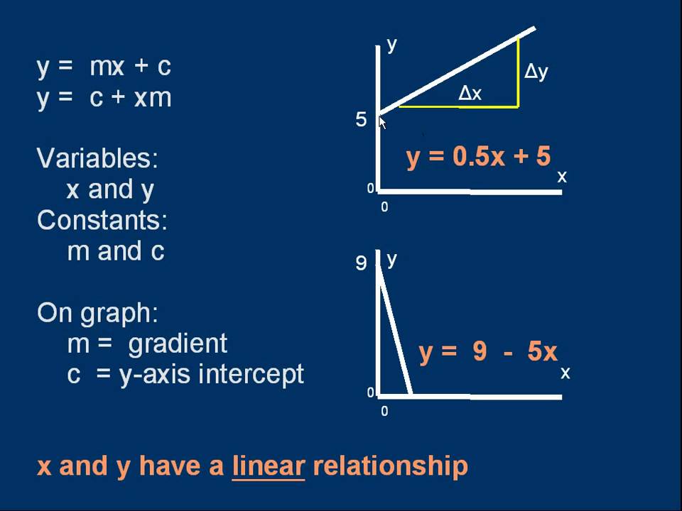
The equation y = mx + c is the cornerstone of linear equations, a fundamental concept in mathematics. But what does it all mean? Let’s break it down. ‘y’ and ‘x’ are variables representing coordinates on a graph. ‘c’ is the y-intercept, the point where the line crosses the y-axis. And ‘m’… ‘m’ is the gradient. The gradient, often called the slope, describes the steepness and direction of a line. It tells you how much ‘y’ changes for every unit change in ‘x’. Mastering the gradient unlocks a deeper understanding of linear relationships and their applications in the real world.
Why is the Gradient Important?
Think about it: the gradient isn’t just a number; it’s a powerful descriptor. Imagine a hill: the gradient tells you how steep the climb will be. In construction, it determines the angle of a roof. In economics, it can represent the rate of change in a supply and demand curve. Understanding how to calculate the gradient empowers you to analyze and interpret linear relationships in countless scenarios.
This guide will provide you with several methods to determine the gradient (‘m’) from the equation y=mx+c. Whether you have the equation, two points on the line, or a graph, we’ll cover the techniques you need to master.
Method 1: When the Equation is in y = mx + c Form
The simplest scenario is when your equation is already neatly arranged in the slope-intercept form: y = mx + c. In this case, finding the gradient is as easy as identifying the coefficient of ‘x’. The number directly multiplying ‘x’ is your ‘m’, the gradient.
Examples
- Example 1: y = 3x + 2. The gradient, m, is 3. This means for every 1 unit increase in ‘x’, ‘y’ increases by 3 units. The line is sloping upwards.
- Example 2: y = -2x + 5. The gradient, m, is -2. This indicates that for every 1 unit increase in ‘x’, ‘y’ decreases by 2 units. The line is sloping downwards.
- Example 3: y = (1/2)x – 1. The gradient, m, is 1/2 or 0.5. This means for every 1 unit increase in ‘x’, ‘y’ increases by 0.5 units. The line has a gentler upward slope.
Rearranging the Equation
Sometimes, the equation isn’t initially in the perfect y = mx + c format. Don’t worry! A little algebraic manipulation will do the trick. The goal is to isolate ‘y’ on one side of the equation. Here’s how:
- Isolate the ‘y’ term: Use addition or subtraction to move any other terms to the opposite side of the equation.
- Divide to get ‘y’ alone: If ‘y’ has a coefficient (a number multiplying it), divide both sides of the equation by that coefficient.
Example:
Let’s say you have the equation 2y + 4x = 6. To find the gradient:
- Subtract 4x from both sides: 2y = -4x + 6
- Divide both sides by 2: y = -2x + 3
Now the equation is in y = mx + c form. The gradient, m, is -2.
Method 2: Finding the Gradient from Two Points
Another common scenario is finding the gradient when you’re given two points on the line. Each point is represented by coordinates (x1, y1) and (x2, y2). The formula to calculate the gradient is:
m = (y2 – y1) / (x2 – x1)
In simpler terms, the gradient is the change in ‘y’ divided by the change in ‘x’. It’s the rise over the run.
Steps to Calculate the Gradient
- Identify the coordinates: Determine the (x, y) values for both points. Label them (x1, y1) and (x2, y2). It doesn’t matter which point you choose as (x1, y1) and which you choose as (x2, y2), as long as you are consistent.
- Apply the formula: Substitute the values into the formula m = (y2 – y1) / (x2 – x1).
- Simplify: Perform the subtraction and division to find the value of ‘m’.
Examples
- Example 1: Find the gradient of the line passing through the points (1, 2) and (4, 8).
- Let (x1, y1) = (1, 2) and (x2, y2) = (4, 8)
- m = (8 – 2) / (4 – 1) = 6 / 3 = 2
- The gradient, m, is 2.
- Example 2: Find the gradient of the line passing through the points (-2, 3) and (1, -3).
- Let (x1, y1) = (-2, 3) and (x2, y2) = (1, -3)
- m = (-3 – 3) / (1 – (-2)) = -6 / 3 = -2
- The gradient, m, is -2.
- Example 3: Find the gradient of the line passing through the points (0, 5) and (3, 5).
- Let (x1, y1) = (0, 5) and (x2, y2) = (3, 5)
- m = (5 – 5) / (3 – 0) = 0 / 3 = 0
- The gradient, m, is 0. This indicates a horizontal line.
Important Note: Undefined Gradient
If x1 = x2, the denominator (x2 – x1) will be zero. Division by zero is undefined. In this case, the gradient is undefined, and the line is vertical.
Method 3: Finding the Gradient from a Graph
When you have a graph of the line, you can visually determine the gradient. This method relies on identifying two clear points on the line and then calculating the rise over the run.
Steps to Determine the Gradient Graphically
- Identify two points: Choose two distinct points on the line where the coordinates are easy to read. These points should ideally lie on the intersection of grid lines for accurate reading.
- Draw a right triangle: Imagine a right triangle with the line segment between your chosen points as the hypotenuse. The vertical side of the triangle represents the ‘rise’ (change in y), and the horizontal side represents the ‘run’ (change in x).
- Measure the rise and run: Determine the length of the vertical side (rise) and the horizontal side (run). Pay attention to the scale of the graph.
- Calculate the gradient: Divide the rise by the run: m = rise / run.
- Determine the sign: If the line slopes upwards from left to right, the gradient is positive. If the line slopes downwards from left to right, the gradient is negative.
Examples
Imagine a line on a graph. You choose two points: (1, 1) and (3, 5).
- The rise is the difference in the y-coordinates: 5 – 1 = 4
- The run is the difference in the x-coordinates: 3 – 1 = 2
- The gradient is rise / run = 4 / 2 = 2
- Since the line slopes upwards, the gradient is positive. Therefore, m = 2.
If, on the other hand, you chose points where the line sloped downwards, you’d have a negative rise, resulting in a negative gradient.
Handling Different Scales
Be mindful of the scale on the graph’s axes. If the x-axis has a scale of 1 unit per grid line, but the y-axis has a scale of 2 units per grid line, you need to account for this when measuring the rise and run. For instance, if the rise appears to be 2 grid lines, but each grid line represents 2 units on the y-axis, the actual rise is 2 * 2 = 4 units.
Special Cases: Horizontal and Vertical Lines
Two special cases deserve attention: horizontal and vertical lines. They have unique properties related to their gradients.
Horizontal Lines
A horizontal line is perfectly flat. The ‘y’ value remains constant regardless of the ‘x’ value. This means the change in ‘y’ is always zero. Therefore, the gradient of a horizontal line is always 0.
Equation: y = c (where ‘c’ is a constant)
Vertical Lines
A vertical line is perfectly upright. The ‘x’ value remains constant regardless of the ‘y’ value. This means the change in ‘x’ is always zero. Since division by zero is undefined, the gradient of a vertical line is undefined. Vertical lines have an infinite slope; they are infinitely steep.
Equation: x = c (where ‘c’ is a constant)
Practical Applications of the Gradient
The concept of the gradient extends far beyond the classroom. It’s a powerful tool for analyzing and interpreting real-world situations. Here are some examples:
- Physics: The gradient can represent the velocity of an object. If you plot distance against time, the gradient of the line at any point gives you the object’s instantaneous velocity.
- Engineering: Engineers use gradients to design roads, bridges, and buildings. The gradient of a road determines its steepness, while the gradient of a roof affects water runoff.
- Economics: As mentioned earlier, gradients can represent the rate of change in supply and demand curves. They can also be used to analyze cost functions and profit margins.
- Geography: Topographic maps use contour lines to represent elevation. The gradient between contour lines indicates the steepness of the terrain.
- Computer Graphics: Gradients are used in shading and lighting models to create realistic images.
Common Mistakes to Avoid
When working with gradients, it’s easy to make mistakes. Here are some common pitfalls to watch out for:
- Inconsistent Subtraction: When using the two-point formula, ensure you subtract the y-coordinates and x-coordinates in the same order. Don’t do (y2 – y1) / (x1 – x2).
- Incorrect Sign: Pay attention to the sign of the gradient. A positive gradient indicates an upward slope, while a negative gradient indicates a downward slope.
- Ignoring the Scale: When finding the gradient from a graph, remember to account for the scale of the axes.
- Undefined Gradient: Remember that vertical lines have an undefined gradient, not a gradient of zero.
- Confusing Slope and Intercept: Make sure you correctly identify ‘m’ as the slope and ‘c’ as the y-intercept in the equation y = mx + c.
Advanced Concepts: Parallel and Perpendicular Lines
The gradient also provides valuable information about the relationship between two lines. Specifically, it tells us whether the lines are parallel or perpendicular.
Parallel Lines
Parallel lines have the same gradient. This means they have the same steepness and direction. They will never intersect.
If line 1 has a gradient of m1 and line 2 has a gradient of m2, then the lines are parallel if m1 = m2.
Perpendicular Lines
Perpendicular lines intersect at a right angle (90 degrees). The gradients of perpendicular lines have a special relationship: they are negative reciprocals of each other.
If line 1 has a gradient of m1 and line 2 has a gradient of m2, then the lines are perpendicular if m1 * m2 = -1, or m2 = -1/m1.
In other words, to find the gradient of a line perpendicular to a given line, flip the fraction (take the reciprocal) and change the sign.
Example
If a line has a gradient of 2/3, then a line perpendicular to it will have a gradient of -3/2.
Practice Problems
To solidify your understanding of gradients, here are some practice problems:
- Find the gradient of the line y = 5x – 3.
- Find the gradient of the line 3y + 6x = 9.
- Find the gradient of the line passing through the points (2, 4) and (5, 10).
- Find the gradient of the line passing through the points (-1, -2) and (3, -2).
- A line has a gradient of -1/4. What is the gradient of a line perpendicular to it?
- Find the equation of the line passing through the point (0,2) and parallel to the line y = 3x + 1.
Answers to Practice Problems
- m = 5
- m = -2
- m = 2
- m = 0
- m = 4
- y = 3x + 2
Conclusion
Understanding how to find the gradient is a crucial skill in mathematics and beyond. Whether you’re given the equation in slope-intercept form, two points on the line, or a graph, the techniques outlined in this guide will empower you to confidently determine the gradient. Remember to practice regularly and pay attention to common mistakes. With a solid understanding of gradients, you’ll be well-equipped to tackle a wide range of mathematical and real-world problems. So go forth, calculate those slopes, and unlock the power of linear relationships!
