Unveiling Excel’s Secrets: A Comprehensive Guide to Finding and Eliminating Duplicate Data

The Frustration of Duplicate Data

Let’s be honest, we’ve all been there. You’re staring at a spreadsheet, a sea of numbers, names, and data, and a nagging feeling creeps in: are there duplicates lurking within? Duplicate data in an Excel file can be a real headache. It can skew your analysis, lead to inaccurate conclusions, and waste valuable time. Imagine trying to analyze sales figures only to find that the same transaction is listed multiple times. Or, think about the implications of sending multiple emails to the same customer. It’s not a pretty picture.

This guide is designed to be your comprehensive companion in the fight against duplicate data. We’ll delve into the various methods Excel offers to identify and eliminate duplicates, from the simple to the more advanced. Whether you’re a seasoned Excel pro or a complete beginner, you’ll find techniques and tips to streamline your data cleaning process. We’ll also explore the potential pitfalls and offer solutions to common challenges. So, buckle up, and let’s get started on our journey to a cleaner, more accurate Excel experience!

Why Identifying and Removing Duplicates Matters

Before we dive into the ‘how,’ let’s briefly touch upon the ‘why.’ Understanding the importance of removing duplicates will further motivate you to master these techniques. Here’s a breakdown of the key benefits:

• Data Accuracy: Duplicate entries can lead to incorrect calculations and skewed results. Removing them ensures your data reflects reality.
• Efficient Analysis: Clean data allows for faster and more accurate analysis, saving you time and effort.
• Improved Decision-Making: Reliable data leads to better informed decisions. The insights you glean from your data will be more trustworthy.
• Enhanced Productivity: Working with clean data reduces frustration and allows you to focus on more important tasks.
• Avoiding Errors: Duplicates can result in errors, such as over-counting, incorrect totals, and misleading averages.

In essence, cleaning up your data is an investment in the quality of your work and the reliability of your results. It’s about making sure your data is trustworthy and useful.

Method 1: Using Excel’s Built-in ‘Remove Duplicates’ Feature

This is arguably the easiest and most straightforward method for removing duplicates. It’s a quick and dirty way to get rid of redundant entries, especially when you’re dealing with a relatively small dataset. Here’s how it works:

1. Select Your Data: Highlight the range of cells that you want to check for duplicates. This can be a single column, multiple columns, or the entire spreadsheet.
2. Go to the ‘Data’ Tab: In the Excel ribbon, click on the ‘Data’ tab.
3. Find ‘Remove Duplicates’: In the ‘Data Tools’ group, you’ll see a button labeled ‘Remove Duplicates.’ Click on it.
4. The ‘Remove Duplicates’ Dialog Box: A dialog box will appear. This is where you specify which columns you want to check for duplicates. By default, Excel selects all columns in your selected range.
5. Choose Your Columns: Check the boxes next to the column headers that you want to use to identify duplicates. For example, if you want to find duplicates based on ‘First Name’ and ‘Last Name,’ make sure those boxes are checked. If you only want to find duplicates based on one column, select only that column.
6. ‘My data has headers’: If your data has a header row, ensure the box ‘My data has headers’ is checked. This is important because it tells Excel to exclude the header row from the duplicate check.
7. Click ‘OK’: Excel will analyze your data based on your selections and remove any duplicate rows. A message box will appear telling you how many duplicates were removed and how many unique values remain.

Important Considerations for ‘Remove Duplicates’:

• Data Loss: The ‘Remove Duplicates’ feature permanently deletes the duplicate rows. Make sure you have a backup copy of your data if you’re unsure.
• Exact Matches: This feature looks for exact matches across the selected columns. If there are slight variations (e.g., a space at the end of a name), it might not identify them as duplicates.
• Column Selection: Carefully choose the columns that define a duplicate. For example, if you’re checking for duplicate customers, you might select ‘First Name,’ ‘Last Name,’ and ‘Email Address.’

This method is ideal for a quick cleanup, but it’s not always the best choice for complex scenarios. Let’s move on to a more versatile approach.

Method 2: Utilizing Conditional Formatting to Highlight Duplicates

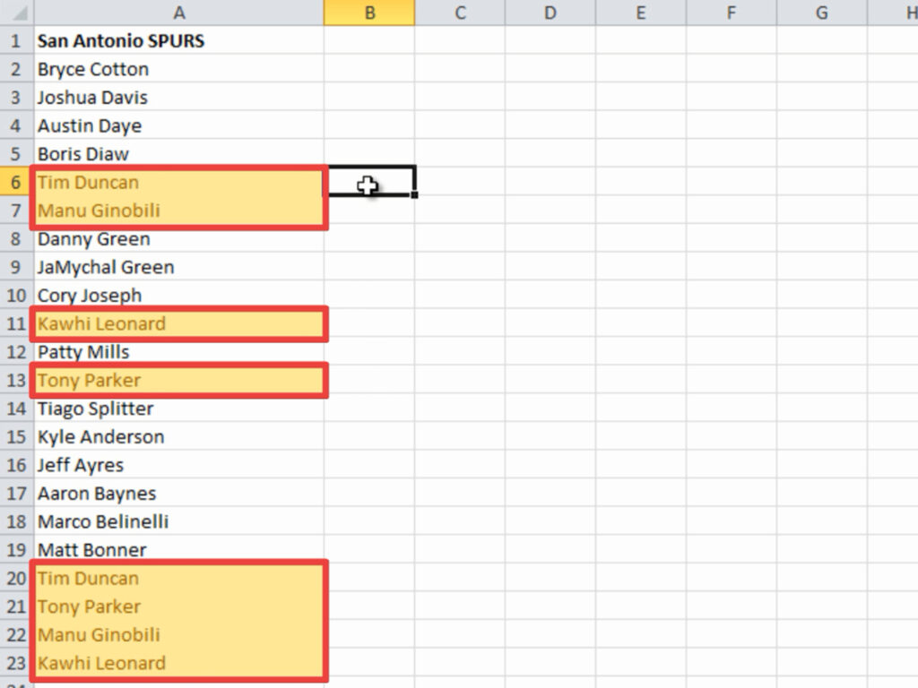
This method is an excellent way to visually identify duplicates without deleting any data. It uses Excel’s conditional formatting feature to highlight duplicate entries, making them stand out. This is particularly useful if you want to review the duplicates before deciding whether to remove them.

1. Select Your Data: Select the range of cells you want to check for duplicates.
2. Go to the ‘Home’ Tab: Click on the ‘Home’ tab in the Excel ribbon.
3. Find ‘Conditional Formatting’: In the ‘Styles’ group, click on ‘Conditional Formatting.’
4. Choose ‘Highlight Cells Rules’: A dropdown menu will appear. Select ‘Highlight Cells Rules.’
5. Select ‘Duplicate Values’: In the ‘Highlight Cells Rules’ submenu, choose ‘Duplicate Values.’
6. Choose Your Formatting: A dialog box will appear. Here, you can choose how you want to highlight the duplicate values. You can select from pre-defined formats (e.g., light red fill with dark red text) or create your own custom format.
7. Click ‘OK’: Excel will apply the conditional formatting, highlighting all duplicate values in your selected range.

Benefits of Conditional Formatting:

• Visual Identification: Easily spot duplicates at a glance.
• No Data Loss: Your original data remains intact.
• Review and Edit: Allows you to review the duplicates and decide how to handle them (e.g., correct errors, merge entries, or remove them later).
• Flexibility: You can customize the formatting to suit your needs.

This method is great for a quick visual check and for identifying potential errors in your data. Remember that the highlighting only shows you the duplicates; you still need to decide what to do with them.

Method 3: Employing the ‘Advanced Filter’ for Duplicate Identification

The ‘Advanced Filter’ is a powerful tool that offers more control over filtering and data manipulation. While it doesn’t directly remove duplicates, it allows you to extract a list of unique values, which can be a great starting point for further analysis and cleaning.

1. Select Your Data: Select the range of cells that contains the data you want to analyze.
2. Go to the ‘Data’ Tab: Click on the ‘Data’ tab in the Excel ribbon.
3. Find ‘Advanced’: In the ‘Sort & Filter’ group, click on the ‘Advanced’ button.
4. The ‘Advanced Filter’ Dialog Box: A dialog box will appear.
5. Choose ‘Filter the list, in-place’ or ‘Copy to another location’: You have two options:
   • ‘Filter the list, in-place’: This will filter the original data, showing only the unique values.
   • ‘Copy to another location’: This will copy the unique values to a different location, leaving your original data untouched. This is generally the safer and more recommended option.
6. Specify the List range: The ‘List range’ should already be populated with the range of cells you selected in step 1. If not, you can manually enter the range or click the icon to select it.
7. Check ‘Unique records only’: Crucially, check the box next to ‘Unique records only.’ This tells Excel to extract only the unique values.
8. Specify the Copy to location (if applicable): If you chose ‘Copy to another location,’ specify the cell where you want the unique values to be copied.
9. Click ‘OK’: Excel will either filter the original data to show only unique values (if you chose ‘Filter the list, in-place’) or copy the unique values to the specified location (if you chose ‘Copy to another location’).

Advantages of the Advanced Filter:

• Control: Offers more control over the filtering process.
• Data Preservation: Allows you to extract unique values without modifying the original data.
• Flexibility: Can be used to filter based on multiple criteria and create more complex data subsets.

This method is particularly useful when you need to create a separate list of unique values for further analysis or reporting.

Method 4: Using Formulas to Identify and Manage Duplicates

Excel formulas provide a powerful and flexible way to identify and manage duplicates. While this method requires a bit more technical know-how, it offers a high degree of control and can handle more complex scenarios. Let’s explore some key formulas:

1. COUNTIF Function

The COUNTIF function is a fundamental tool for identifying duplicates. It counts the number of times a specific value appears within a range. Here’s how to use it:

1. Select an Empty Column: Choose an empty column next to your data (e.g., column D if your data is in column C).
2. Enter the Formula: In the first cell of the empty column (e.g., D1), enter the following formula: =COUNTIF(C:C, C1). Replace ‘C:C’ with the column containing the data you want to check for duplicates. Replace ‘C1’ with the first cell in the column you are checking.
3. Drag the Formula Down: Click and drag the small square in the bottom-right corner of the cell down to apply the formula to all the rows in your data.

Interpreting the Results: The formula will return a number for each cell in the empty column. If the number is greater than 1, it indicates a duplicate. For example, if a cell shows ‘2,’ it means the value in the corresponding row appears twice in the column. If the result is ‘1,’ it means the value is unique in that column.

2. Using COUNTIF with Conditional Formatting

You can combine the COUNTIF function with conditional formatting to visually highlight duplicates, as described earlier. This is a powerful way to automate the process.

1. Apply the COUNTIF formula (as described above).
2. Select Your Data: Select the range of cells containing the data.
3. Go to the ‘Home’ Tab: Click on the ‘Home’ tab in the Excel ribbon.
4. Find ‘Conditional Formatting’: In the ‘Styles’ group, click on ‘Conditional Formatting.’
5. Choose ‘New Rule’: In the dropdown, select ‘New Rule.’
6. Select ‘Use a formula to determine which cells to format’: In the ‘New Formatting Rule’ dialog box, select this option.
7. Enter the Formula: In the ‘Format values where this formula is true’ box, enter the formula: =COUNTIF(C:C, C1)>1. Replace ‘C:C’ with the column containing the data and ‘C1’ with the first cell in the column.
8. Click ‘Format’: Click the ‘Format’ button to choose the formatting you want to apply to the duplicates (e.g., fill color, font color).
9. Click ‘OK’ twice: Click ‘OK’ in the ‘Format Cells’ dialog box and then again in the ‘New Formatting Rule’ dialog box.

Now, any cell with a duplicate value in your data will be highlighted based on the formatting you selected.

3. The UNIQUE Function (Excel 365 and Later)

For users of Excel 365 and later, the UNIQUE function provides a simpler and more elegant way to extract unique values. This function automatically returns a list of unique values from a range.

1. Select an Empty Column: Choose an empty column where you want the unique values to appear.
2. Enter the Formula: In the first cell of the empty column, enter the formula: =UNIQUE(C:C). Replace ‘C:C’ with the column containing the data you want to check for duplicates.
3. The Unique Values: The formula will automatically populate the cells below with the unique values from the specified column.

Advantages of Formula-Based Methods:

• Flexibility: Formulas can be adapted to handle a wide range of scenarios and complex criteria.
• Automation: Formulas automatically update as your data changes.
• Control: You have complete control over the logic used to identify duplicates.

While these methods may require a bit of practice, they offer the most powerful and versatile solutions for identifying and managing duplicates in Excel.

Method 5: Leveraging Power Query for Advanced Duplicate Handling

For users who work with large datasets or need more advanced data manipulation, Power Query (also known as Get & Transform Data) offers a powerful and efficient solution for identifying and removing duplicates. Power Query is a built-in data transformation and connection tool in Excel.

1. Import Your Data: If your data is already in Excel, select the data range and go to the ‘Data’ tab. Click on ‘From Table/Range’ in the ‘Get & Transform Data’ group. If your data is from an external source (e.g., a text file or database), use the appropriate import options in the ‘Get & Transform Data’ group.
2. The Power Query Editor: The Power Query Editor window will open. This is where you’ll perform the duplicate removal.
3. Select the Columns: In the Power Query Editor, select the column(s) you want to check for duplicates.
4. Remove Duplicates: Go to the ‘Home’ tab in the Power Query Editor. In the ‘Reduce Rows’ group, click on ‘Remove Rows’ and then select ‘Remove Duplicates.’
5. Review and Refine: Power Query will remove the duplicate rows based on your selection. Review the results in the editor.
6. Load the Results: Click ‘Close & Load’ in the ‘Home’ tab to load the cleaned data back into your Excel worksheet.

Advantages of Using Power Query:

• Efficiency: Power Query is optimized for handling large datasets.
• Data Transformation: Offers a wide range of data transformation capabilities, including cleaning, shaping, and merging data.
• Automation: You can save your steps as a query, allowing you to refresh the data and automatically remove duplicates whenever the data changes.
• Connection to External Data: Power Query can connect to various data sources, making it ideal for working with data from databases, cloud services, and other sources.

Power Query is a valuable tool for anyone who works with large datasets and needs a robust solution for data cleaning and transformation.

Troubleshooting Common Duplicate Issues

Even with the best methods, you might encounter some challenges. Here are some common issues and how to address them:

• Inconsistent Data Entry: Typos, variations in capitalization, and extra spaces can prevent duplicates from being identified.
  • Solution: Use the TRIM function to remove extra spaces, the UPPER or LOWER functions to standardize capitalization, and the SUBSTITUTE function to correct typos.
• Hidden Characters: Non-printing characters (e.g., line breaks) can also cause problems.
  • Solution: Use the CLEAN function to remove these characters.
• Partial Duplicates: Sometimes, you might have partial duplicates, where some columns match but others don’t.
  • Solution: Carefully select the columns to use for identifying duplicates and consider using formulas or Power Query to combine data from multiple columns.
• Data Format Issues: Ensure your data is in the correct format (e.g., dates, numbers). Incorrect formatting can lead to unexpected results.

By addressing these potential issues, you can ensure that your duplicate identification and removal processes are as accurate and effective as possible.

Best Practices for Preventing Duplicate Data

Prevention is always better than cure. Here are some best practices to minimize the occurrence of duplicate data in the first place:

• Data Validation: Use data validation rules to restrict the type of data that can be entered in a cell. This can help prevent typos and inconsistencies.
• Drop-Down Lists: Use drop-down lists to limit the choices available for data entry. This reduces the risk of variations in spelling or formatting.
• Consistent Formatting: Establish and enforce consistent formatting rules for your data.
• Data Entry Templates: Use data entry templates to standardize the data entry process.
• Training and Documentation: Train users on proper data entry procedures and provide clear documentation.
• Regular Data Audits: Regularly review your data for duplicates and other errors.

By implementing these preventive measures, you can significantly reduce the need to clean up duplicate data in the future.

Conclusion: Mastering the Art of Duplicate Data Management in Excel

Finding and removing duplicates in Excel is a fundamental skill for anyone who works with data. Whether you’re a student, a business professional, or a data analyst, understanding these techniques can save you time, improve accuracy, and enhance your decision-making abilities. From the simple ‘Remove Duplicates’ feature to the more advanced formulas and Power Query, Excel offers a variety of tools to meet your specific needs. By mastering these methods and implementing best practices, you can transform your spreadsheets from a source of frustration into a powerful tool for analysis and insight. Embrace the power of clean data, and watch your productivity and the quality of your work soar! Remember to choose the method that best suits your data and your level of expertise. Don’t be afraid to experiment and practice. The more you work with these techniques, the more comfortable and efficient you’ll become. Happy data cleaning!